Writing a decision tree from scratch
Decision Trees are pretty cool. I started learning about DTs from Jeremy Howard's ML course and found them fascinating. In order to gain deeper insights into DTs, I decided to build one from scratch. This notebook/blog-post is a summary of that exercise.
I wanted to start blogging about DTs (and Data Science in general) once I became adept in the field, but after reading this FCC article I've decided to get into it early. So let's get to it.
A few good things about DTs are: - Since they're based on a white box model, they're simple to understand and to interpret. - DTs can be visualised. - Requires little data preparation. - Able to handle both numerical and categorical data.
I'll be using the ID3 algorithm to generate the DT.
ID3 uses Entropy and Information Gain to generate trees. I'll get into the details of the two while implementing them.
Let's code this up in Python. I'll be using the titanic dataset from Kaggle.
Table of Contents
Setup
# imports
import pandas as pd
import numpy as np
import math
import random
import uuid
from IPython.display import Image
from sklearn.tree import DecisionTreeClassifier
from sklearn import tree
import pydot
from sklearn.model_selection import train_test_split
import graphviz
from numpy import array
import pprint
from fastai.structured import train_cats, proc_df
import matplotlib.pyplot as plt
import six
DATA_PATH = 'data/titanic/'
data = pd.read_csv(f'{DATA_PATH}train.csv')
This is how the original data looks.
data.head()

For the sake of simplicity, I'm dropping NA rows.
data.dropna(axis=0,inplace=True)
Since I'm trying to replicate the functionality of a DT from scratch, I'd like to start with a small dataset with a small number of columns.
data1 = data[:30]
'Name', 'Ticket', and 'PassengerId' are mostly useless for me here. Dropping 'Cabin', 'Embarked', and 'Fare' to keep things simple.
titanic1 = data1.drop(['Name','Ticket','PassengerId','Cabin','Age','Embarked','Fare'],axis=1)
Okay. This is how the data looks like now.
titanic1.head()

ID3 implementation
Time to code up the metrics. I'll start with the most naive versions of them, with very less focus on optimisation.
Entropy
Entropy H(S) is a measure of the amount of uncertainty in the (data) set S.
$${H(S)=\sum\limits_{x \in X}-p(x)\log_{2}p(x)}$$
Where, - S – The current (data) set for which entropy is being calculated (changes every iteration of the ID3 algorithm) - X – Set of classes in S - p(x) – The proportion of the number of elements in class x to the number of elements in set S
When entropy=0, the set S is perfectly classified (i.e. all elements in S are of the same class).
def entropy(data,y_field):
    # data is a pandas DataFrame
    sum = 0
    for el in data[y_field].value_counts():
        prob = el/len(data)
        sum += prob*math.log(prob,2)
    sum*=-1
    return sum
Information Gain
Information gain IG(A) is the measure of the difference in entropy from before to after the set S is split on an attribute A. In other words, how much uncertainty in S was reduced after splitting set S on attribute A.
$$IG(A,S)=H(S)-\sum\limits_{t \in T}p(t)H(t)$$
Where,
- H(S) – Entropy of set S
- T – The subsets created from splitting set S by attribute A
- p(t) – The proportion of the number of elements in t to the number of elements in set S
- H(t) – Entropy of subset t
def info_gain(data,attribute,y_field):
    current_entropy = entropy(data,y_field)
    uniques = data[attribute].value_counts().keys()
    sec_term = 0
    for i,cat_count in enumerate(data[attribute].value_counts()):
        sec_term += (cat_count/len(data))*entropy(data[data[attribute]==uniques[i]],y_field)
    entropy_for_attribute = current_entropy - sec_term
    return entropy_for_attribute
Okay, now that we have the two metrics implemented, time to write a simple function that builds a tree. It finds the best column to split on using the above two metrics, and recusively generates the tree as a Python dictionary. Recursion stops when all elements in a node belong to a single class.
def build_tree(data,y_field,level=0,tree=None,verbose=False):
    cols = list(data.columns)
    cols.remove(y_field)
    info_gains = []
    for col in cols:
        info_gains.append(round(info_gain(data,col,y_field),2))
    if verbose:
        print(cols,info_gains)
    if(len(set(info_gains))==1): #all info gains are zero
#         choose the decision as the output with a higher count
        col_to_split_on = random.choice(cols)
        values_to_split_on = data[col_to_split_on].unique()
        node = col_to_split_on
        if tree is None:
            tree = {}
            tree[node] = {}
        for value in values_to_split_on:
            sub_df = data[data[col_to_split_on]==value]
            if verbose:
                print(f'No info gain, uniques: {sub_df[y_field].unique()}')
            most_frequent = sub_df[y_field].mode()[0]
            if verbose:
                print(f'Setting {col_to_split_on} with value {value} as leaf with output {most_frequent}')
            tree[node][str(value)] = str(most_frequent)
    else:
        col_to_split_on = cols[info_gains.index(max(info_gains))]
        values_to_split_on = data[col_to_split_on].unique()
    #         print(col_to_split_on)
        node = col_to_split_on
        if tree is None:
            tree = {}
            tree[node] = {}
        for value in values_to_split_on:
            sub_df = data[data[col_to_split_on]==value]
            if verbose:
                print(f'Level->{level},total_cols:{cols}, Split on {col_to_split_on} on value {value}, uniques:{sub_df[y_field].unique()}')
            if len(sub_df[y_field].unique())==1:
    #             print(f'level->{level},{value},leaf')
                tree[node][str(value)] = str(sub_df[y_field].unique()[0])
                if verbose:
                    print(f'Level->{level}, Reached leaf for {col_to_split_on} at value {value} with output {sub_df[y_field].unique()[0]}')
            else:
#                 x = input('go deeper?\n')
                x = 'y'
                if x !='n':
                    tree[node][str(value)] = build_tree(sub_df,y_field,level=level+1,verbose=verbose)
                else:
                    tree[node][str(value)]=None
    return tree
my_tree = build_tree(titanic1[:20],'Survived',verbose=True)
['Pclass', 'Sex', 'SibSp', 'Parch'] [0.11, 0.49, 0.04, 0.01]
Level->0,total_cols:['Pclass', 'Sex', 'SibSp', 'Parch'], Split on Sex on value female, uniques:[1]
Level->0, Reached leaf for Sex at value female with output 1
Level->0,total_cols:['Pclass', 'Sex', 'SibSp', 'Parch'], Split on Sex on value male, uniques:[0 1]
['Pclass', 'Sex', 'SibSp', 'Parch'] [0.2, 0.0, 0.1, 0.03]
Level->1,total_cols:['Pclass', 'Sex', 'SibSp', 'Parch'], Split on Pclass on value 1, uniques:[0 1]
['Pclass', 'Sex', 'SibSp', 'Parch'] [0.0, 0.0, 0.09, 0.03]
Level->2,total_cols:['Pclass', 'Sex', 'SibSp', 'Parch'], Split on SibSp on value 0, uniques:[0 1]
['Pclass', 'Sex', 'SibSp', 'Parch'] [0.0, 0.0, 0.0, 0.0]
No info gain, uniques: [0 1]
Setting SibSp with value 0 as leaf with output 0
Level->2,total_cols:['Pclass', 'Sex', 'SibSp', 'Parch'], Split on SibSp on value 3, uniques:[0]
Level->2, Reached leaf for SibSp at value 3 with output 0
Level->2,total_cols:['Pclass', 'Sex', 'SibSp', 'Parch'], Split on SibSp on value 1, uniques:[0]
Level->2, Reached leaf for SibSp at value 1 with output 0
Level->1,total_cols:['Pclass', 'Sex', 'SibSp', 'Parch'], Split on Pclass on value 2, uniques:[1]
Level->1, Reached leaf for Pclass at value 2 with output 1
Level->1,total_cols:['Pclass', 'Sex', 'SibSp', 'Parch'], Split on Pclass on value 3, uniques:[0]
Level->1, Reached leaf for Pclass at value 3 with output 0
Okay. So the function seems to work. One of the best things about a DT is that it can be visualized pretty easily. Let's do that. I'll use the awesome graphviz tool and pydot to visualize the tree.
def walk_dictionaryv2(graph, dictionary, parent_node=None):
    for k in dictionary.keys():

        if parent_node is not None:

            from_name = parent_node.get_name().replace("\"", "") + '_' + str(k)
            from_label = str(k)
            obj_dict = {}

            if 'True' in from_label:
                node_from = pydot.Node(from_name, color='white', style='filled',fillcolor='green', label=from_label)
            elif 'False' in from_label:
                node_from = pydot.Node(from_name, color='white', style='filled',fillcolor='red', label=from_label)
            else:
                node_from = pydot.Node(from_name, label=from_label)

            graph.add_node(node_from)

            graph.add_edge( pydot.Edge(parent_node, node_from) )

            if isinstance(dictionary[k], dict): # if interim node
                walk_dictionaryv2(graph, dictionary[k], node_from)

            else: # if leaf node
                to_name = str(uuid.uuid4()) + '_' + str(dictionary[k]) # unique name
                to_label = str(dictionary[k])

                node_to = pydot.Node(to_name, label=to_label, shape='box')
                graph.add_node(node_to)
                graph.add_edge(pydot.Edge(node_from, node_to))
        else:

            from_name =  str(k)
            from_label = str(k)

            node_from = pydot.Node(from_name, label=from_label)
            walk_dictionaryv2(graph, dictionary[k], node_from)


def plot_tree(tree, name):
    graph = pydot.Dot(graph_type='graph')
    walk_dictionaryv2(graph, tree)
    graph.write_png(name+'.png')
plot_tree(my_tree,'1')
Image(filename='1.png',unconfined=True)
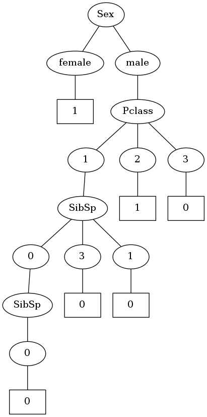
Okay! So I did manage to create a decision tree. Although it doesn't quite look like a traditional decision tree where nodes represent columns and edges represent values. I'm not gonna bother with that for now. In this version, one node represents the column to split on and the following node represents the value taken.
But I can see one problem with this kind of structure. As per this implementation of classic ID3, one node will be split into as many child nodes as the number of unique values that node can have. So in the above tree, Pclass is split into 3 child nodes as it can take the values 1,2,3.
I intentionally didn't use the columns which can take continous values for creating this tree. Let's add the column age to our dataframe.
titanic2 = data1.drop(['Name','Ticket','PassengerId','Cabin','Embarked','Fare'],axis=1)
titanic2.head()

my_tree = build_tree(titanic2[:20],'Survived',verbose=False)
plot_tree(my_tree,'2')
Image(filename='2.png',unconfined=True)
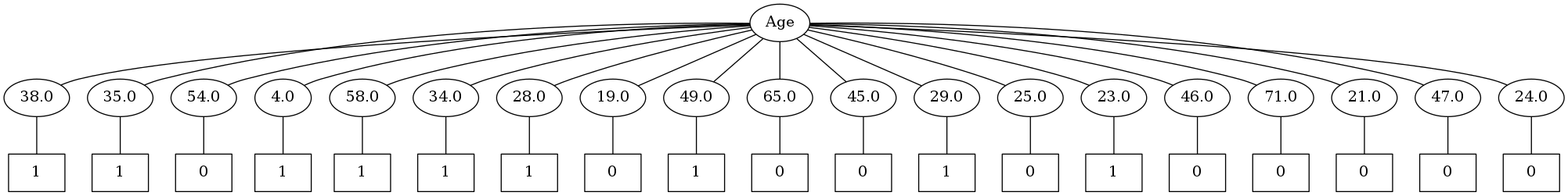
Oh boy. It seems that this algorithm will have a tough time with continous values. Time to tweak it so as to handle continous values properly by doing binary splits. This is the default implementation of decision trees in scikit-learn.
Binary Splits
Entropy implementation remains the same.
def entropy(data,y_field):
    # data is a pandas DF
    sum = 0
    for el in data[y_field].value_counts():
        prob = el/len(data)
        sum += prob*math.log(prob,2)
    sum*=-1
    return sum
Information Gain implementation has to be changed a little. Instead of iterating over all possible values for a column, I'll just use a split point to create two subsets. And since I'm using a split point, which is a number, the entire dataset will have to be converted into numerical values. I'll do it later.
def info_gain_for_binary(data,attribute,mid_point,y_field):
    current_entropy = entropy(data,y_field)
    uniques = data[attribute].value_counts().keys()
    sec_term = 0
#     since it's a binary split, need to find entropy for just two sub-dataframes created from a split point
    sec_term += (len(data[data[attribute]<mid_point])/len(data))*entropy(data[data[attribute]<mid_point],y_field)
    sec_term += (len(data[data[attribute]>=mid_point])/len(data))*entropy(data[data[attribute]>=mid_point],y_field)
    entropy_for_attribute = current_entropy - sec_term
    return entropy_for_attribute
find_best_split takes a dataframe and finds the split which results in maximum info gain. Basically it iterates over all columns, and all possible midpoints of the values of a column and finds the best split.
Note to self: A lot of optimisation pending here.
def find_best_split(data,y_field,verbose=False):
    cols = list(data.columns)
    cols.remove(y_field)
    info_gains = []
    splits = []
    for attribute in cols:
        data2 = data.sort_values(by=attribute,axis=0)
        vals = np.array(data2[attribute].unique())
        if len(vals)>1:
    #   https://stackoverflow.com/questions/23855976/middle-point-of-each-pair-of-an-numpy-array
            mid_points = (vals[1:] + vals[:-1]) / 2
            info_gains_for_attribute = []
            for mid_point in mid_points:
                info_gains_for_attribute.append(info_gain_for_binary(data2,attribute,mid_point,y_field))
            best_split_point_for_attribute = mid_points[info_gains_for_attribute.index(max(info_gains_for_attribute))]
            info_gains.append(max(info_gains_for_attribute))
            splits.append(best_split_point_for_attribute)
        else:
            splits.append(vals[0])
            info_gains.append(info_gain_for_binary(data2,attribute,vals[0],y_field))
    if verbose:
        print(cols,info_gains)
    max_val = max(info_gains)
    max_at = [i for i, x in enumerate(info_gains) if x == max_val]
    max_at_index = random.choice(max_at)
    best_col_to_split_on = cols[max_at_index]
    best_split_value = splits[max_at_index]
    return (best_col_to_split_on,best_split_value)
build_tree_binary is similar to the previous build_tree, the only difference being it only creates two subsets based on a split point.
Condition used to split on is "less than or equal to". So, the elements satisfying this condition are placed in the imaginary left node, and the others in the right one.
# intuition: for each column, sort it, create mid points for each pair of values, iterate
# over those values, and check
def build_tree_binary(data,y_field,level=0,tree=None,verbose=False):
#     print(data.columns)
    if verbose:
        print('\n\n---------\n\n')
        print(f'Samples: {len(data)}')
    best_col_to_split_on,best_split_value = find_best_split(data,y_field,verbose=verbose)
    if verbose:
        print(f'Level-{level}. Split on {best_col_to_split_on} at value {best_split_value}')

    node = f'{best_col_to_split_on}<={best_split_value}'
    if tree is None:
        tree = {}
        tree[node] = {}

    sub_df_left = data[data[best_col_to_split_on]<=best_split_value]
    sub_df_right = data[data[best_col_to_split_on]>best_split_value]
    if len(sub_df_left[y_field].unique())==1:
        if verbose:
            print(f'Reached node on left at level {level+1}')
        tree[node]['True'] = str(sub_df_left[y_field].unique()[0])
    else:
#         x = input(f'Left at level {level+1}')
        tree[node]['True'] = build_tree_binary(sub_df_left,y_field,level=level+1,verbose=verbose)

    if len(sub_df_right[y_field].unique())==1:
        if verbose:
            print(f'Reached node on right at level {level+1}')
        tree[node]['False'] = str(sub_df_right[y_field].unique()[0])
    else:
#         x = input(f'Right at level {level+1}')
        tree[node]['False'] = build_tree_binary(sub_df_right,y_field,level=level+1,verbose=verbose)

    return tree
titanic3 = data1.drop(['Name','Ticket','PassengerId','Cabin','Embarked'],axis=1)
Okay, so I'm using some functions from the fastai library to prepare the dataset for building the tree. train_cats converts string columns to columns of categorical values. proc_df splits off the response variable, and changes the dataframe into an entirely numeric one.
train_cats(titanic3)
df, y, nas = proc_df(titanic3, 'Survived')
dft1 = df.copy()
dft1['Survived'] = y
%%time
tsttree = build_tree_binary(dft1[:20],'Survived',verbose=False)
CPU times: user 584 ms, sys: 8 ms, total: 592 ms
Wall time: 578 ms
plot_tree(tsttree,'3')
Image(filename='3.png',unconfined=True)
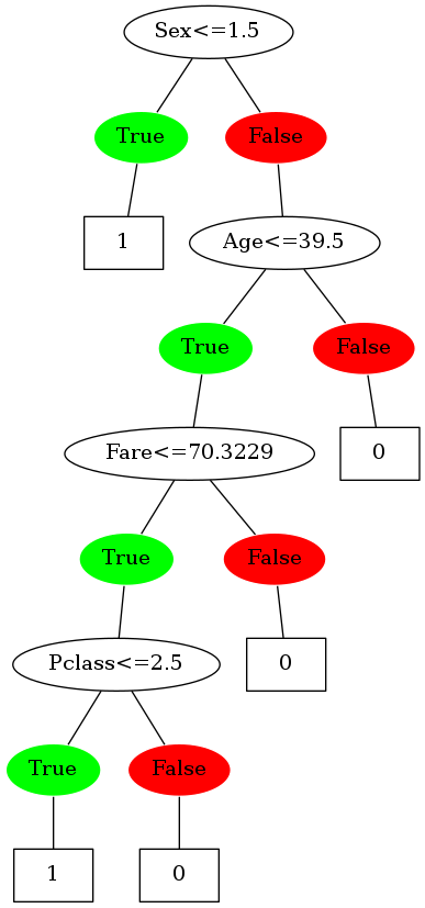
Sweet! The tree is now making binary splits. Time to compare it with the scikit-learn version of the DT. (Not in terms of performance obviously, just on the basis of the decisions it's making)
dt = DecisionTreeClassifier(criterion='entropy')
dt.fit(df[:20],y[:20])
DecisionTreeClassifier(class_weight=None, criterion='entropy', max_depth=None,
            max_features=None, max_leaf_nodes=None,
            min_impurity_decrease=0.0, min_impurity_split=None,
            min_samples_leaf=1, min_samples_split=2,
            min_weight_fraction_leaf=0.0, presort=False, random_state=None,
            splitter='best')
dot_data = tree.export_graphviz(dt, out_file=None,
                         feature_names=list(df.columns),
                         class_names=['Not eat','Eat'],
                         filled=True, rounded=True,
                         special_characters=True)
graph = graphviz.Source(dot_data)
graph.format = 'png'
graph.render()
Image(filename='Source.gv.png',unconfined=True)
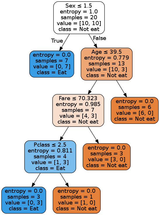
Boo-yaa! Our tree is making the same decisions as the scikit-learn's tree.
One point to note here though: Since the dataset is very small, as we approach the leaf nodes, different splits will result in same information gains. So the decisions near the bottom of the tree may vary as I randomly choose a column to split on in the case of same info gains.
Prediction
def predict_binary_one_row(row,tree):
    for node in tree.keys():
        els = node.split('<=')
        col = els[0]
        split_point =  float(els[1])
        value = row[col]
        if value <= split_point:

            tree = tree[node]['True']
        else:
            tree = tree[node]['False']
        prediction = None

        if type(tree) is dict:
            prediction = predict_binary_one_row(row, tree)
        else:
            prediction = tree
            break;

    return prediction

def predict_binary(df,tree):
    rows = df.to_dict('records')
    predictions = []
    for row in rows:
        prediction = predict_binary_one_row(row,tree)
        predictions.append(int(prediction))
    return predictions
def rmse(x,y): return math.sqrt(((x-y)**2).mean())
rmse(predict_binary(dft1[20:30],tsttree),y[20:30])
0.5477225575051661
This is the first version of the ID3 DT written from scratch. Obviously, things can be sped up a lot by making use of numpy and vectorization. But my aim for this exercise was to understand the underlying logic used to build a DT, and creating one from scratch definitely facilitated that.
Next, I'll be building a DT using the CART algorithm.