Understanding ResNets

I'm currently enrolled in fastai's Deep Learning MOOC (version 3), and loving it so far. It's only been 2 lectures as of today, but folks are already building awesome stuff based on the content taught so far.

The course starts with the application of DL in Computer Vision, and in the very first lecture, course instructor Jeremy teaches us how to leverage transfer learning by making use of pre-trained ResNet models. I've been meaning to dive into the details of Resnets for a while, and this seems like a good time to do so.

This post is written in the vein of a summary-note, rather than that of a full-fledged introduction to resnets, ie, it's (sort-of) written for my own future reference, and can be helpful for somebody with some background on the topic.

What problems did the residual learning framework try to solve?¶

Network depth is of crucial importance in "very-deep" convolutional neural networks as seen in best performing models in ILSVRC since 2012. But stacking more layers to plain feed forward networks results in degradation of training accuracy.

He et al. write in their paper:

When deeper networks are able to start converging, a degradation problem has been exposed: with the network depth increasing, accuracy gets saturated and then degrades rapidly. Unexpectedly, such degradation is not caused by overfitting, and adding more layers to a suitably deep model leads to higher training error.

This degradation problem has been verified by experiments, and can be seen in the following figure.

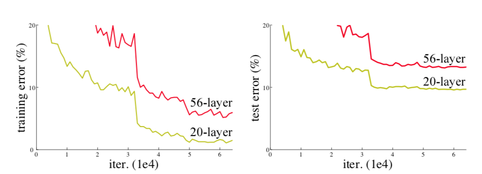
So that's the problem resets tried to solve, ie, optimizing very deep networks without running into degradation, and to also do it in feasible time.

How did the residual learning framework solve these problems?¶

The degradation (of training accuracy) indicates that not all systems are similarly easy to optimize. Let us consider a shallower architecture and its deeper counterpart that adds more layers onto it.

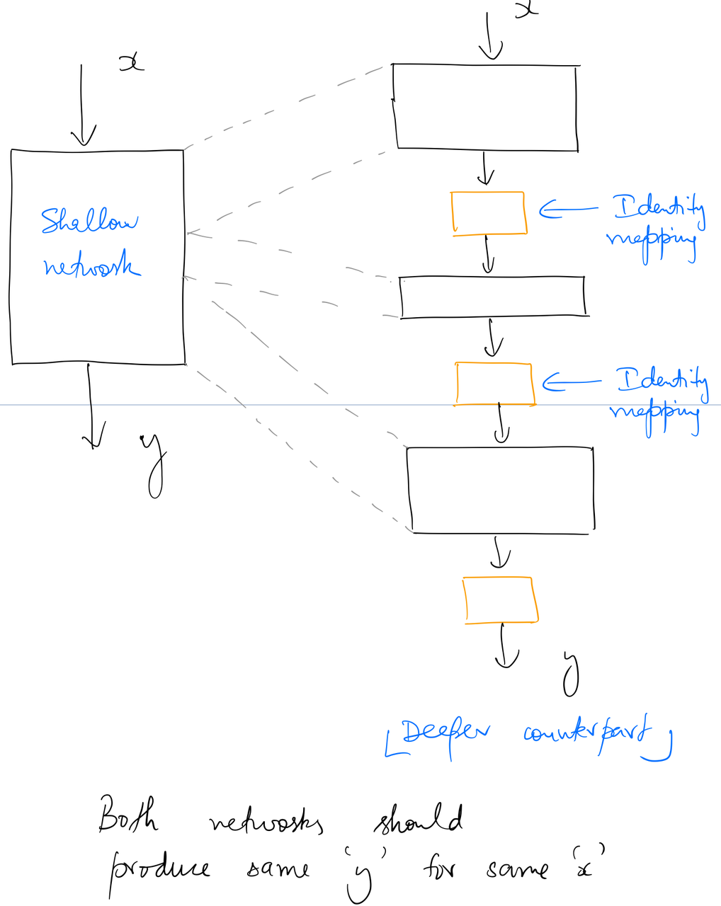
There exists a solution by construction to the deeper model: the added layers are identity mapping, and the other layers are copied from the learned shallower model. The existence of this constructed solution indicates that a deeper model should produce no higher training error than its shallower counterpart. But experiments show that our current solvers on hand are unable to find solutions that are comparably good or better than the constructed solution (or unable to do so in feasible time).

The crux of the deep residual learning framework can be summarised in this line from the paper:

Instead of hoping each few stacked layers directly fit a desired underlying mapping, we explicitly let these layers fit a residual mapping.

What does this mean?¶

Instead of making a network deeper by simply stacking layers to it, He et al. suggest using a residual block.

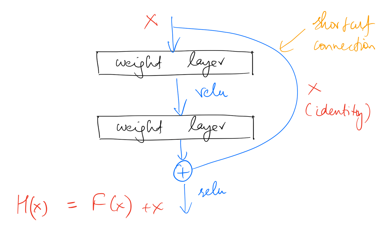
Here, we want the block to learn to output $H(x)$ when x is input to it. Instead of stacking identity mapping between the weight layers, we add a identity mapping shortcut connection as shown the figure above. Without the shortcut connection, the stacked layers would've outputted $F(x)$. Due to the shortcut connection being an identity mapping, the stacked non-linear layers now learn to output a new $F(x) = H(x) - x$.

We hypothesize that it is easier to optimize the residual mapping than to optimize the original, unreferenced mapping. To the extreme, if an identity mapping were optimal, it would be easier to push the residual to zero than to fit an identity mapping by a stack of nonlinear layers.

In real cases, it is unlikely that identity mappings are optimal, but our reformulation may help to precondition the problem. If the optimal function [$H(x)$] is closer to an identity mapping than to a zero mapping, it should be easier for the solver to find the perturbations with reference to an identity mapping, than to learn the function as a new one. We show by experiments that the learned residual functions in general have small responses, suggesting that identity mappings provide reasonable preconditioning.

Anand Saha has a superb explanation of 'residual' on his blog, as follows:

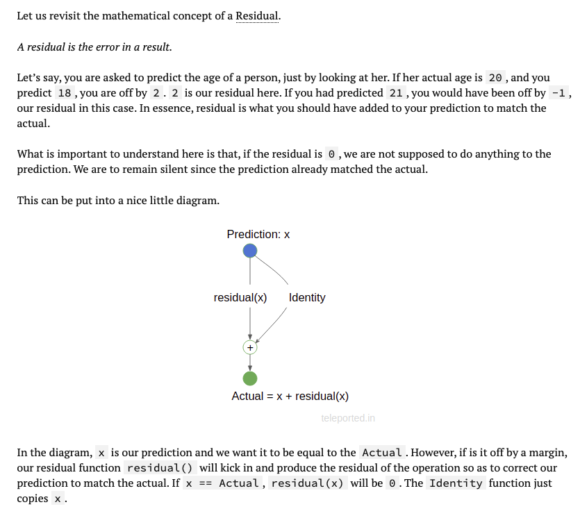
So simply put, residual learning makes it easier for the solvers to efficiently adjust the weight layers to optimise the network. Now we know the intuition behind the residual learning framework. Let's dig into Resnet implementation. I'll be exploring two variants: ResNet-34, and ResNet-50, comprising 34 and 50 layers respectively.

Identity and Projection shortcuts¶

The residual block that I've drawn above has a shortcut connection that is an identity mapping. This is true if the shapes of the input and output tensors of the block are same. If that's not the case, residual blocks use something called a projection shortcut, which involves a convolution (and a Batch Norm) that alters the shape of the input tensor to match that of the output. We'll see that in action below.

Basic residual block¶

ResNets can be built using two kinds of block implementations, basic block and bottleneck block, explained in detail below.

Notation: I'll be referring to channels (in images) as planes. Also, the word "dimensions" in the figures below explicitly mean the height and width of feature maps. So when I say, dimensions halve, I'm only referring to the height and width of the feature maps, and not the planes.

I'll use Pytorch's implementation as reference. Let's take a look at basic residual block's implementation.

class BasicBlock(nn.Module):
    expansion = 1

    def __init__(self, inplanes, planes, stride=1, downsample=None):
        super(BasicBlock, self).__init__()
        self.conv1 = conv3x3(inplanes, planes, stride)
        self.bn1 = nn.BatchNorm2d(planes)
        self.relu = nn.ReLU(inplace=True)
        self.conv2 = conv3x3(planes, planes)
        self.bn2 = nn.BatchNorm2d(planes)
        self.downsample = downsample
        self.stride = stride

    def forward(self, x):
        residual = x

        out = self.conv1(x)
        out = self.bn1(out)
        out = self.relu(out)

        out = self.conv2(out)
        out = self.bn2(out)

        if self.downsample is not None:
            residual = self.downsample(x)

        out += residual
        out = self.relu(out)

        return out

So a basic residual block has two convolutional layers, each using 3*3 filters. The stride of the first conv can be 1 or 2 (as we'll see) but the second conv is always 1. Also, a downsampling (via projection shortcut) is done whenever required.

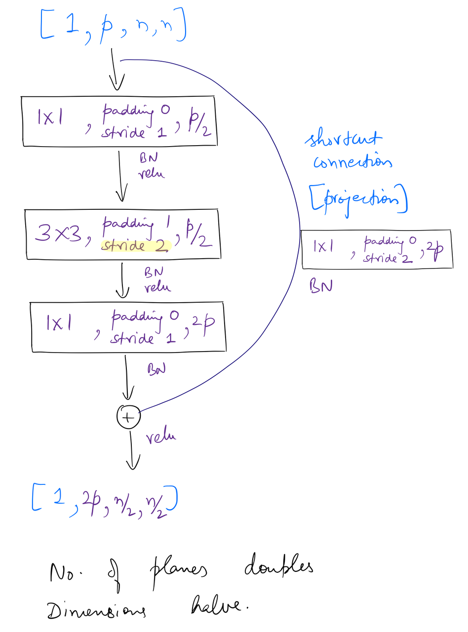
After going through the complete network architecture, I found the following two variants of the basic block used in ResNet-34. We haven't seen the ResNet-34 architecture yet, but understanding how these blocks are used in it can be helpful. (of course, going back and forth never harms)

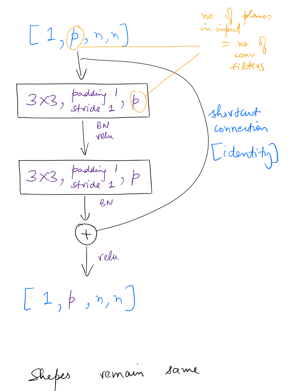
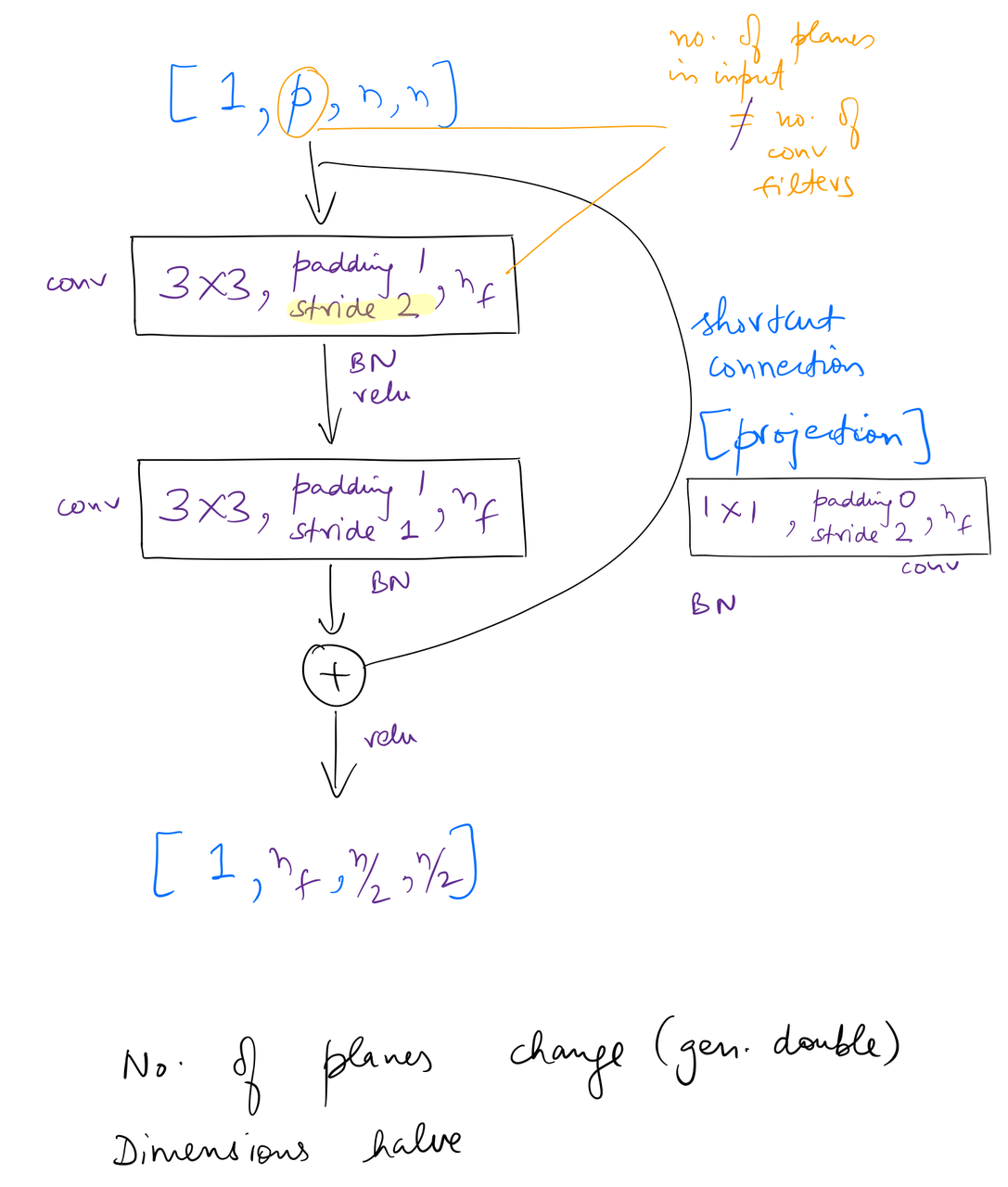
So in the first variant, the shapes of the input and output tensors remain same, while in the second variant shapes change. More specifically, in the second variant, the number of planes change (generally double, as we'll see below), and the dimensions of feature maps halve.

Let's see this basic block in action. Below is PyTorch's implementation of a ResNet.

class ResNet(nn.Module):

    def __init__(self, block, layers, num_classes=1000):
        self.inplanes = 64
        super(ResNet, self).__init__()
        self.conv1 = nn.Conv2d(3, 64, kernel_size=7, stride=2, padding=3,
                               bias=False)
        self.bn1 = nn.BatchNorm2d(64)
        self.relu = nn.ReLU(inplace=True)
        self.maxpool = nn.MaxPool2d(kernel_size=3, stride=2, padding=1)
        self.layer1 = self._make_layer(block, 64, layers[0])
        self.layer2 = self._make_layer(block, 128, layers[1], stride=2)
        self.layer3 = self._make_layer(block, 256, layers[2], stride=2)
        self.layer4 = self._make_layer(block, 512, layers[3], stride=2)
        self.avgpool = nn.AdaptiveAvgPool2d((1, 1))
        self.fc = nn.Linear(512 * block.expansion, num_classes)

        for m in self.modules():
            if isinstance(m, nn.Conv2d):
                nn.init.kaiming_normal_(m.weight, mode='fan_out', nonlinearity='relu')
            elif isinstance(m, nn.BatchNorm2d):
                nn.init.constant_(m.weight, 1)
                nn.init.constant_(m.bias, 0)

    def _make_layer(self, block, planes, blocks, stride=1):
        downsample = None
        if stride != 1 or self.inplanes != planes * block.expansion:
            downsample = nn.Sequential(
                conv1x1(self.inplanes, planes * block.expansion, stride),
                nn.BatchNorm2d(planes * block.expansion),
            )

        layers = []
        layers.append(block(self.inplanes, planes, stride, downsample))
        self.inplanes = planes * block.expansion
        for _ in range(1, blocks):
            layers.append(block(self.inplanes, planes))

        return nn.Sequential(*layers)

ResNet-34 can be created as follows:

resnet34 = ResNet(BasicBlock, [3, 4, 6, 3])

PyTorch's implementation of a ResNet uses the notation of a "layer". This "layer" is simply residual blocks stacked together, and can be of varying lengths. For ResNet-34, the layers argument is [3, 4, 6, 3]. The base number of planes of these layers are [64, 128, 256, 512].

When applicable _make_layer will downsample the input tensor of the first block for projection shortcuts.

How tensors move through a ResNet-34?¶

The use of the above two variants of the basic block will become more clear once we see how tensors move through a ResNet-34. So see that, I'll make use of PyTorch's forward hook feature.

When the last line is run, it prints out a huge chunk of strings from the hooks attached. To not let it fill up the page, below is a scrollable PDF of the output which is also annotated with my remarks.

Summary for ResNet-34:¶

• Input tensor shape: [1, 3, 224, 224]
• Initial conv:
  • Output: [1, 64, 112, 112]
  • Net result: Planes -> 64, dimensions get halved
• Initial pool:
  • Output: [1, 64, 56, 56]
  • Net result: Dimensions get halved
• Layer 1 (3 blocks)
  • Output: [1, 64, 56, 56]
  • Net result: Planes remains same, dimensions remain same
• Layer 2 (4 blocks)
  • Output: [1, 128, 28, 28]
  • Net result: Planes double, dimensions halve
• Layer 3 (6 blocks)
  • Output: [1, 256, 14, 14]
  • Net result: Planes double, dimensions halve
• Layer 4 (3 blocks)
  • Output: [1, 512, 7, 7]
  • Net result: Planes double, dimensions halve
• Avg pool
  • Output: [1, 512, 1, 1]
• Fully connected:
  • Output: [1, 1000]

So that's how a ResNet-34 works! Let's do the same exercise for ResNet-50.

Bottleneck residual block¶

class Bottleneck(nn.Module):
    expansion = 4

    def __init__(self, inplanes, planes, stride=1, downsample=None):
        super(Bottleneck, self).__init__()
        self.conv1 = conv1x1(inplanes, planes)
        self.bn1 = nn.BatchNorm2d(planes)
        self.conv2 = conv3x3(planes, planes, stride)
        self.bn2 = nn.BatchNorm2d(planes)
        self.conv3 = conv1x1(planes, planes * self.expansion)
        self.bn3 = nn.BatchNorm2d(planes * self.expansion)
        self.relu = nn.ReLU(inplace=True)
        self.downsample = downsample
        self.stride = stride

    def forward(self, x):
        residual = x

        out = self.conv1(x)
        out = self.bn1(out)
        out = self.relu(out)

        out = self.conv2(out)
        out = self.bn2(out)
        out = self.relu(out)

        out = self.conv3(out)
        out = self.bn3(out)

        if self.downsample is not None:
            residual = self.downsample(x)

        out += residual
        out = self.relu(out)

        return out

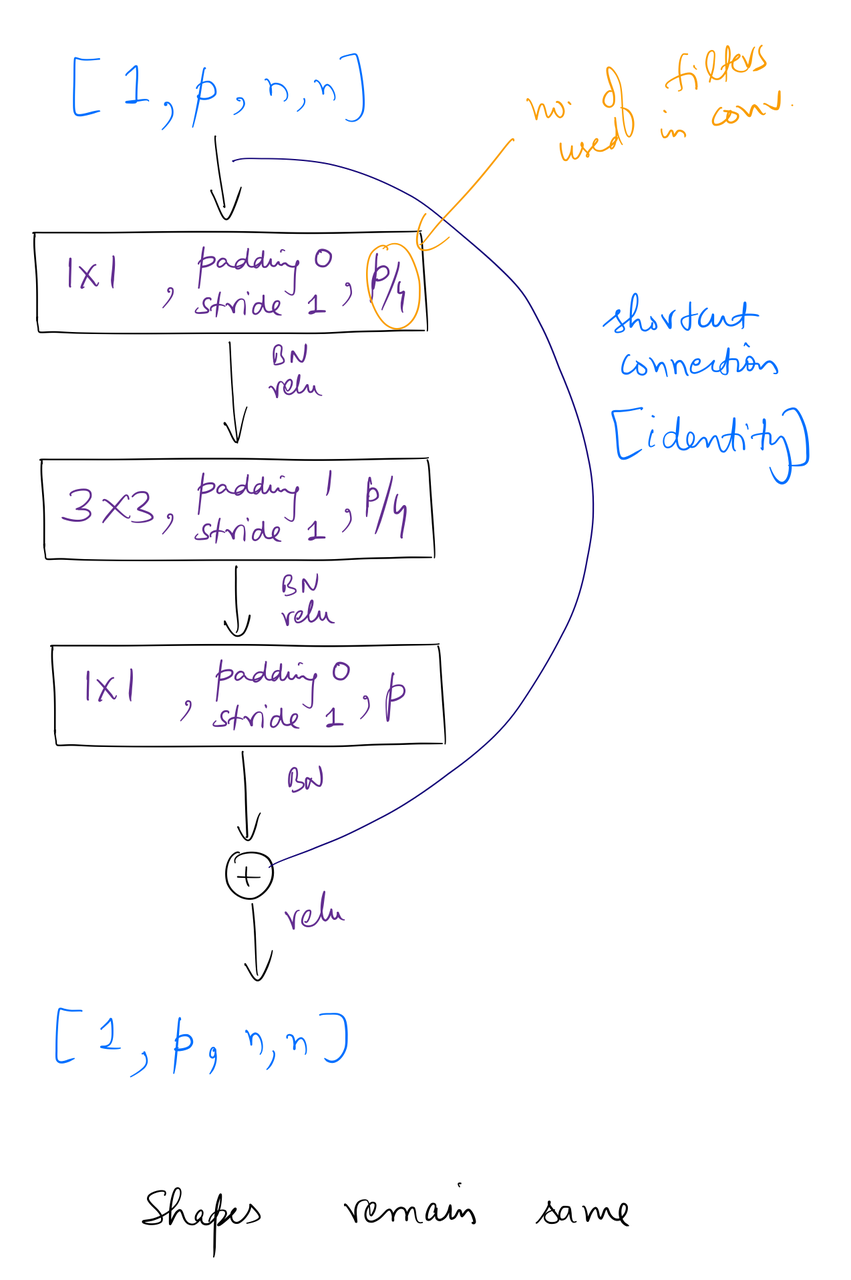
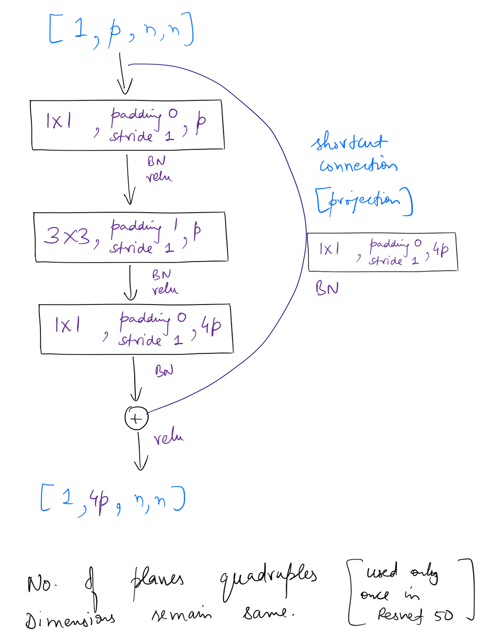
A bottleneck residual block has 3 convolutional layers, using 1*1, 3*3 and 1*1 filter sizes respectively. The stride of the first and second convolutions is always 1, while the second convolution can have a stride of either 1 or 2 (as we'll see). A downsampling (via projection shortcut) is done whenever required. One point to note here is that a bottleneck block has an expansion of 4 (as compared to 1 for basic block).

Similar to the approach above, I found the following two variants of the bottleneck block used in ResNet-50.

ResNet-50 can be created as follows:

resnet34 = ResNet(Bottleneck, [3, 4, 6, 3])

The only difference between the implementations of ResNet-34 and 50 is the kind of block used. Let's run the forward hooks for a ResNet-50.

Again, below is a scrollable PDF of the output of the last line.

Summary for ResNet-50:¶

• Input tensor shape: [1, 3, 224, 224]
• Initial conv:
  • Output: [1, 64, 112, 112]
  • Net result: Planes -> 64, dimensions get halved
• Initial pool:
  • Output: [1, 64, 56, 56]
  • Net result: Dimensions get halved
• Layer 1 (3 blocks)
  • Output: [1, 256, 56, 56]
  • Net result: Planes quadruple, dimensions remain same
• Layer 2 (4 blocks)
  • Output: [1, 512, 28, 28]
  • Net result: Planes double, dimensions halve
• Layer 3 (6 blocks)
  • Output: [1, 1024, 14, 14]
  • Net result: Planes double, dimensions halve
• Layer 4 (3 blocks)
  • Output: [1, 2048, 7, 7]
  • Net result: Planes double, dimensions halve
• Avg pool
  • Output: [1, 2048, 1, 1]
• Fully connected:
  • Output: [1, 1000]

The difference between overall operations of residual layers of ResNet-34 and 50 is seen only in the first layer. Planes remain same in the case of ResNet-34, while in ResNet-50, planes quadruple. After the first layer, for both ResNet-34 and 50, overall operations remain same for each layer, ie, planes double and dimensions halve.

This was a fun (and loong) exercise, but definitely helpful in gaining insights into ResNets.

References:¶

• Deep Residual Learning for Image Recognition
• https://github.com/pytorch/vision/blob/master/torchvision/models/resnet.py
• http://teleported.in/posts/decoding-resnet-architecture/
• https://medium.com/@14prakash/understanding-and-implementing-architectures-of-resnet-and-resnext-for-state-of-the-art-image-cf51669e1624