Summary Notes: GRU and LSTMs
This post is sort-of a continuation to my last post, which was a Summary Note on the workings of basic Recurrent Neural Networks. As I mentioned in that post, I've been learning about the workings of RNNs for the past few days, and how they deal with sequential data, like text. An RNN can be built using either a basic RNN unit (described in the last post), a Gated Recurrent unit, or an LSTM unit. This post will describe how GRUs/LSTMs learn long term dependencies in the data, which is something basic RNN units are not so good at.
This is not an introductory article on the workings of GRU/LSTMs. For that refer to these remarkable articles.
- The Unreasonable Effectiveness of Recurrent Neural Networks by Andrej Karpathy
- Understanding LSTM Networks by Christopher Olah
Learning long-term dependencies
This is how a basic RNN cell looks like:
And these are the forward prop equations: $$a^{\langle t \rangle} = \tanh(W_{aa} a^{\langle t-1 \rangle} + W_{ax} x^{\langle t \rangle} + b_a)$$ $$\hat{y}^{\langle t \rangle} = softmax(W_{ya} a^{\langle t \rangle} + b_y)$$
At time-step $t$, the hidden state $a^{\langle t \rangle}$ and prediction $\hat{y}^{\langle t \rangle}$ both depend upon the hidden state of previous time-step, ie, $a^{\langle t-1 \rangle}$. This conveys that a basic RNN cell should be able to connect previously learned information with the current one, and thus, should be able to use context it learnt quite in the previous timesteps to yield prediction for the current time-step.
Zachary C. Lipton, John Berkowitz, and Charles Elkan state in their paper "A Critical Review of Recurrent Neural Networks for Sequence Learning" this:
(As in Markov models,) any state in a traditional RNN depends only on the current input as well as on the state of the network at the previous time step. However, the hidden state at any time step can contain information from a nearly arbitrarily long context window. This is possible because the number of distinct states that can be represented in a hidden layer of nodes grows exponentially with the number of nodes in the layer. Even if each node took only binary values, the network could represent 2N states where N is the number of nodes in the hidden layer. When the value of each node is a real number, a network can represent even more distinct states.
It turns out though, traditional RNNs don't do so good when the context has to be remembered for a lot of timesteps.
Gated Recurrent Unit
The GRU was introduced in 2014 by Kyunghyun Cho et al, and although LSTMs were introduced a lot earlier (1997) than GRU, I'll explain GRUs first since they can be seen as a simpler version of LSTMs.
A GRU tries to solve the long-term dependency problem by making use of a "memory cell". In theory, this "memory cell" is supposed to keep track of context as the network trains through the time-steps.
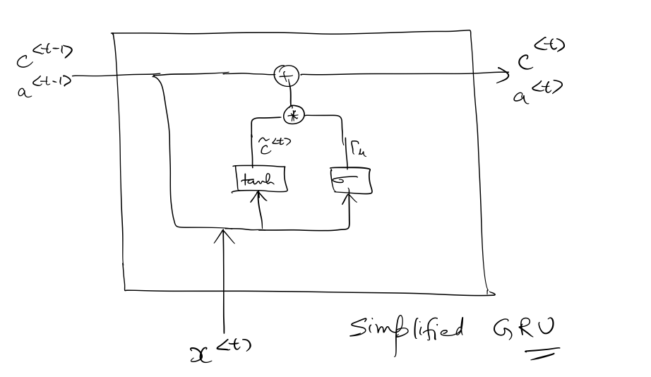
This is how a GRU looks like:
where $c^{\langle t \rangle}$ represents the memory cell for timestep $t$, and is also equal to the hidden state of the GRU, ie, $a^{\langle t \rangle}$.
The size of $c^{\langle t \rangle}$ (as well as $a^{\langle t \rangle}$) depends on the number of hidden units n_a, which is a hyperparameter for the network.
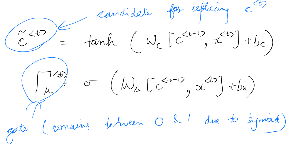
$c^{\langle t \rangle}$ is calculated by first calculating an intermediate value $\tilde{c}^{\langle t \rangle}$, and the update gate $\Gamma_u^{\langle t \rangle}$.
$\Gamma_u^{\langle t \rangle}$ determines the extent to which to forget the previously stored context and also, learn new context from the current time-step. Since $\Gamma_u^{\langle t \rangle}$ is the outcome of a sigmoid operation it's value remains between $0$ and $1$.
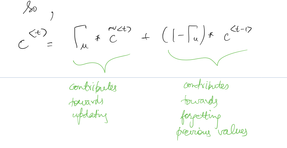
Finally, for time-step $t$:
Since the shape of sigmoid is as follows:
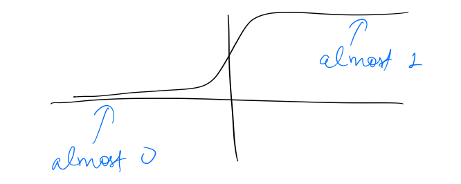 It is easy for the network to set the update gate to zero, ie, $$c^{\langle t \rangle}\approx c^{\langle t-1 \rangle}$$which means that the memory state can be retained over a large number of time-steps. As a result, the network can remember long-term dependencies.
Long Short Term Memory Networks
LSTMs were introduced by Hochreiter & Schmidhuber in 1997, and were specifically designed to learn long-term dependencies. An LSTM unit can be seen as a slighlty more complicated version of the GRU (though technically, a GRU is a simpler version of an LSTM unit).
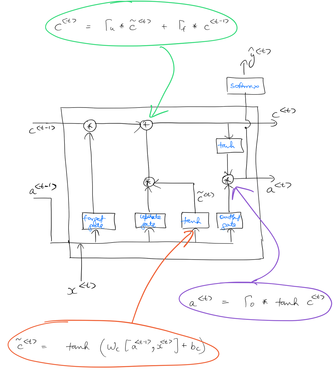
This is how an LSTM unit looks like:
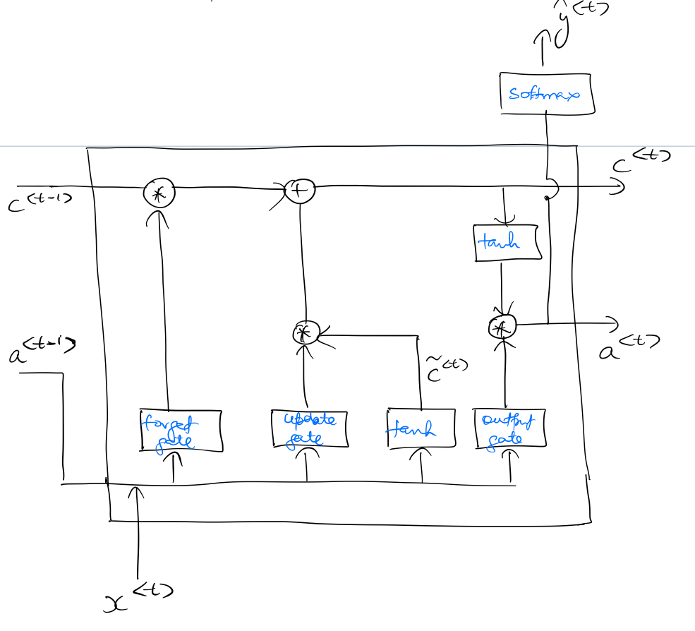
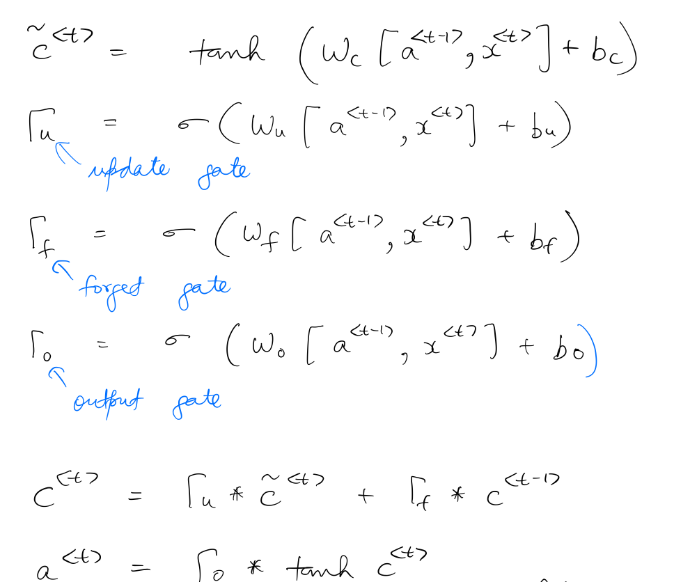
As seen in the above diagram, an LSTM unit has 3 gates (as compared to GRU's one gate) titled forget gate, update gate, and output gate. Unlike GRU, $c^{\langle t \rangle}$, and $a^{\langle t \rangle}$ remain separate entities in an LSTM.
$c^{\langle t \rangle}$, $a^{\langle t \rangle}$, and the gates are calculated as follows:
The following diagram denotes the specific points in the LSTM unit where the calculations are performed.
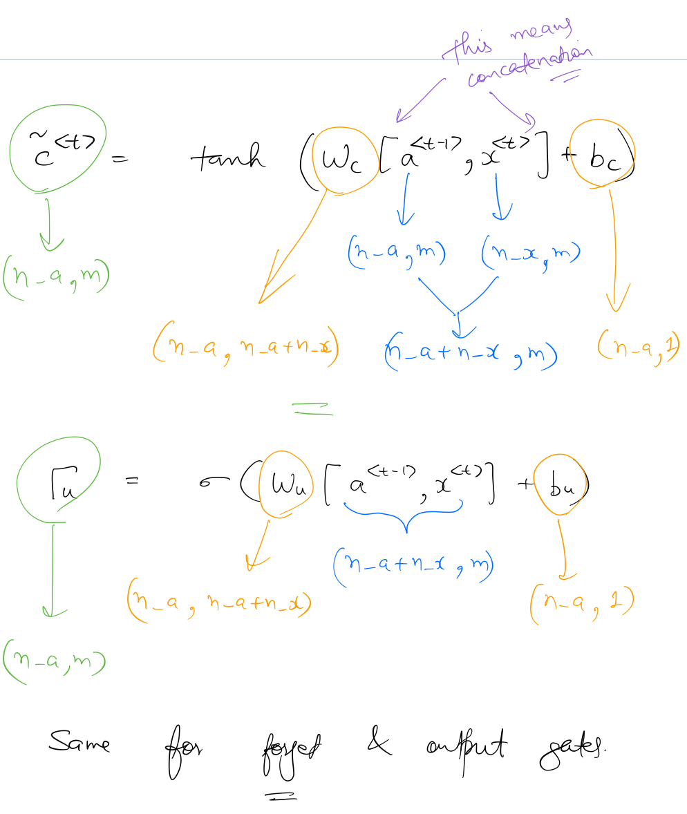
Similar to the convention of a basic RNN unit, $x^{\langle t \rangle}$ is of shape (n_x, m), $a^{\langle t-1 \rangle}$, and $c^{\langle t \rangle}$ are of shape (n_a, m). So the shapes of the gates can be seen as:
So, similar to the GRU, LSTM units are able to learn contexts by making use of the "memory element" $c$. But since LSTM networks have a more robust way of setting the value of $c^{\langle t \rangle}$ (because of the 3 gates), it is generally able to perform better than GRU when it comes to handling long-term dependencies.
LSTMs are also better able to deal with the problem of vanishing and exploding gradients. Lipton et al., 2015 explain this problem in the case of basic RNNs as follows:
As a toy example, consider a network with a single input node, a single output node, and a single recurrent hidden node. Now consider an input passed to the network at time τ and an error calculated at time t, assuming input of zero in the intervening time steps. The tying of weights across time steps means that the recurrent edge at the hidden node j always has the same weight. Therefore, the contribution of the input at time $τ$ to the output at time $t$ will either explode or approach zero, exponentially fast, as $t − τ$ grows large. Hence the derivative of the error with respect to the input will either explode or vanish.
And LSTMs resolve this problem by making use of memory cell:
At the heart of each memory cell is a node $s_c$ [different notation than this post] with linear activation, which is referred to in the original paper as the “internal state” of the cell. The internal state $s_c$ has a self-connected recurrent edge with fixed unit weight [forget gates were not part of the original LSTM design]. Because this edge spans adjacent time steps with constant weight, error can flow across time steps without vanishing or exploding. This edge is often called the constant error carousel.
This constant error carousel enables the gradient to propagate back across many time steps during backpropagation.
References
- deeplearning.ai's Sequence Models course
- A Critical Review of Recurrent Neural Networks for Sequence Learning by Zachary C. Lipton, John Berkowitz, and Charles Elkan
- The Unreasonable Effectiveness of Recurrent Neural Networks by Andrej Karpathy
- Understanding LSTM Networks by Christopher Olah