Summary Notes: Basic Recurrent Neural Networks
I've been learning about Recurrent Neural Nets this week, and this post is a "Summary Note" for the same.
A "Summary Note" is just a blog post version of the notes I make for something, primarily for my own reference (if I need to come back to the material in the future). These summary notes won't go into the very foundations of whatever they're about, but rather serve as a quick and practical reference for that particular topic.
RNNs are inherently different from a traditional feed-forward neural nets, in that, they have the capability to make predictions based on past/future data. This ability to sort of "memorise" past/future data is crucial to handling cases which have a temporal aspect to them. Let's take the following conversation between me and Google Assistant on my phone:

Google Assistant is able to answer my 2nd question even without me explicitly mentioning Lakers in the query (also, it translated stats as 'starts' but that doesn't matter here). It's able to do that because it has the context of what I'm asking it from my previous question. I don't know if Google uses RNNs for this exact functionality but in general RNNs are quite good at this sort of "memorisation" of context. Let's dig into the details of a basic RNN.
Input
The RNN gets $x$ as input.
One input example will span $t$ time-steps, each of which will be denoted as a vector of dimension n_x.
$x^{\langle t \rangle}$ is the input at the $t^{th}$ time-step. $x^{(i)\langle t \rangle}$ is the input at the $t^{th}$ timestep of example $i$.
Output
The RNN will output y which in this example will also span $t$ timesteps, each of which will be a vector of dimension n_y.
Basic RNN cell
This is how a basic RNN cell looks for time step t.
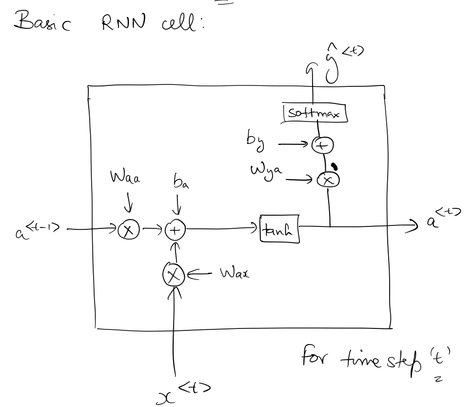
Parameters to learn
So, the parameters that the RNN needs to learn are:
- $W_{ax}$
- $W_{aa}$
- $b_{a}$
- $W_{ya}$
- $b_{y}$
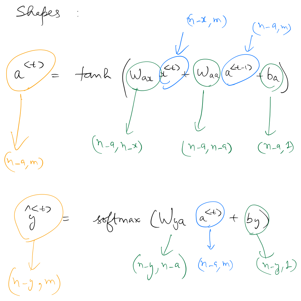
Forward Propagation Equations
Dimensions of $a^{\langle t \rangle}$ and $\hat{y}^{\langle t \rangle}$ are as follows:
Implementation in numpy
# imports and softmax implementation
import numpy as np
import random

def softmax(x):
    e_x = np.exp(x - np.max(x))
    return e_x / e_x.sum(axis=0)
One-hot encoding function. One-hot encodes a number to a column vector of size n_x.
def one_hot_encode(number, n_x):
    x = np.zeros((n_x,1))
    x[number] = 1
    return x
# example
print(one_hot_encode(5,27))
def rnn_step_forward(parameters, a_prev, x):
    """
    One forward propagation step for a basic RNN cell

    Arguments:
    parameters -- python dictionary containing the parameters Waa, Wax, Wya, by, and ba.
    a_prev -- previous hidden state
    x -- input for timestep t

    Returns:
    a_next -- hidden state for time step t
    p_t -- output probabilites

    shapes:
    Waa -- (n_a, n_a)
    Wax -- (n_a, n_x)
    by -- (n_y, 1)
    ba -- (n_a, 1)
    a_prev -- (n_a, m), m=1 in this example
    x -- (n_x,1)
    a_next -- (n_a, m)
    p_t -- (n_a, m)

    """

    Waa, Wax, Wya, by, b = parameters['Waa'], parameters['Wax'], parameters['Wya'], parameters['by'], parameters['ba']
    a_next = np.tanh(np.dot(Wax, x) + np.dot(Waa, a_prev) + ba) # hidden state
    p_t = softmax(np.dot(Wya, a_next) + by)

    return a_next, p_t
def rnn_forward(X, Y, a0, parameters, n_x):
    """
    Forward propagation for RNN

    Arguments:
    X -- python list of one input, eg. [1,2,3,4,5]
    Y -- python list of output corresponding to X, eg. [2,3,4,5,6]
    a0 -- first hidden state (timestep 0)

    Returns:
    loss -- final loss after running through all the time steps
    cache -- tuple of normalized output probabilities, hidden states, and inputs for all time steps
    """

    x, a, y_hat = {}, {}, {}

    a[-1] = np.copy(a0)

    loss = 0

    for t in range(len(X)):

        # Setting x[t] to be the one-hot vector representation of the t'th character in X.

        x[t] = one_hot_encode(t, n_x)

        # Run one step forward of the RNN
        a[t], y_hat[t] = rnn_step_forward(parameters, a[t-1], x[t])

        # Aggregating the loss till the current time step.
        #Update the loss by substracting the cross-entropy term of this time-step from it.
        loss -= np.log(y_hat[t][Y[t],0])

    cache = (y_hat, a, x)

    return loss, cache
Using these equations, hidden states and predictions for each time-step can be calculated. Once forward prop for all the time-steps is complete, we can calculate the gradient of the final prediction wrt loss, and start propagating the gradients back in order to find $\frac{ \partial J } {\partial W_{ax}}, \frac{ \partial J } {\partial W_{aa}}, \frac{ \partial J } {\partial b_{a}}, \frac{ \partial J } {\partial b_{y}}$.
The difference between backpropagation for a feed-forward NN and a RNN is that in case of a RNN, we need to backpropagate through previous time steps (and aggregating the gradients for each timestep in the process), giving it a really cool name, ie, "Backpropagation Through Time".
Backpropagation Through Time
This is how backpropagating through a single time-step looks like. The loss in this case is cross-entropy loss, summed over all time-steps (during forward prop).
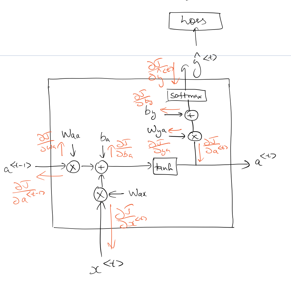
To make things simpler, let's assume we've backpropagated to the point where we've computed $\frac{ \partial J } {\partial a^{\langle t \rangle}}$. This article has a good explanation on backpropagating through a softmax.
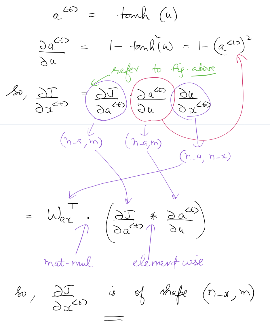
For the sake of simplicity let's define $u^{\langle t \rangle}$ as: $$u^{\langle t \rangle} = W_{aa} a^{\langle t-1 \rangle} + W_{ax} x^{\langle t \rangle} + b_a$$ Once we know $\frac{ \partial J } {\partial a^{\langle t \rangle}}$, we can continue with backpropagation as follows:
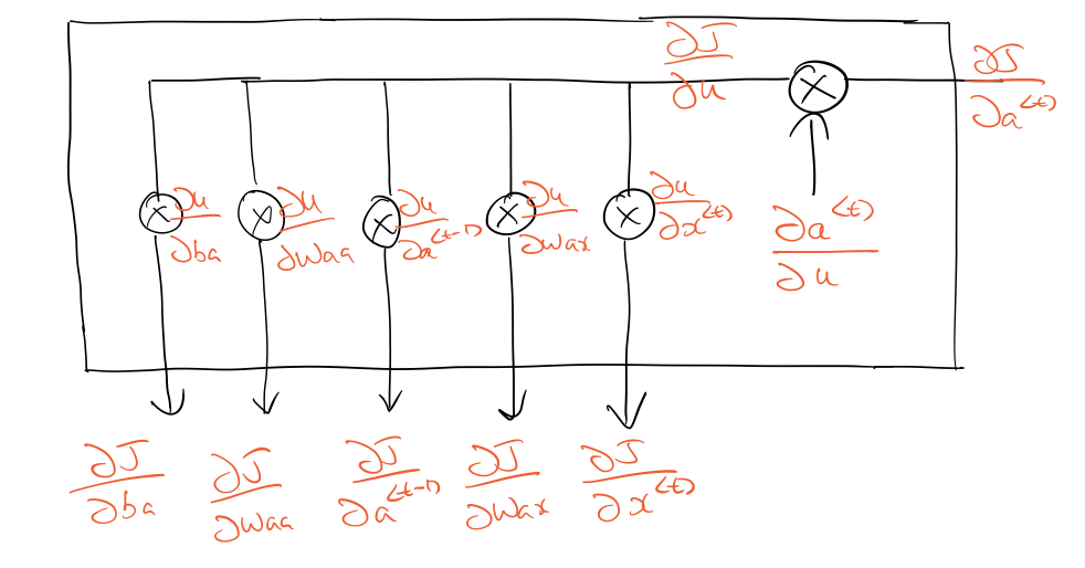
Calculation of $\frac{ \partial J } {x^{\langle t \rangle}}$
Focus on the sequence of multiplications between different tensors which results in the correct dimensions of$\frac{ \partial J } {x^{\langle t \rangle}}$:
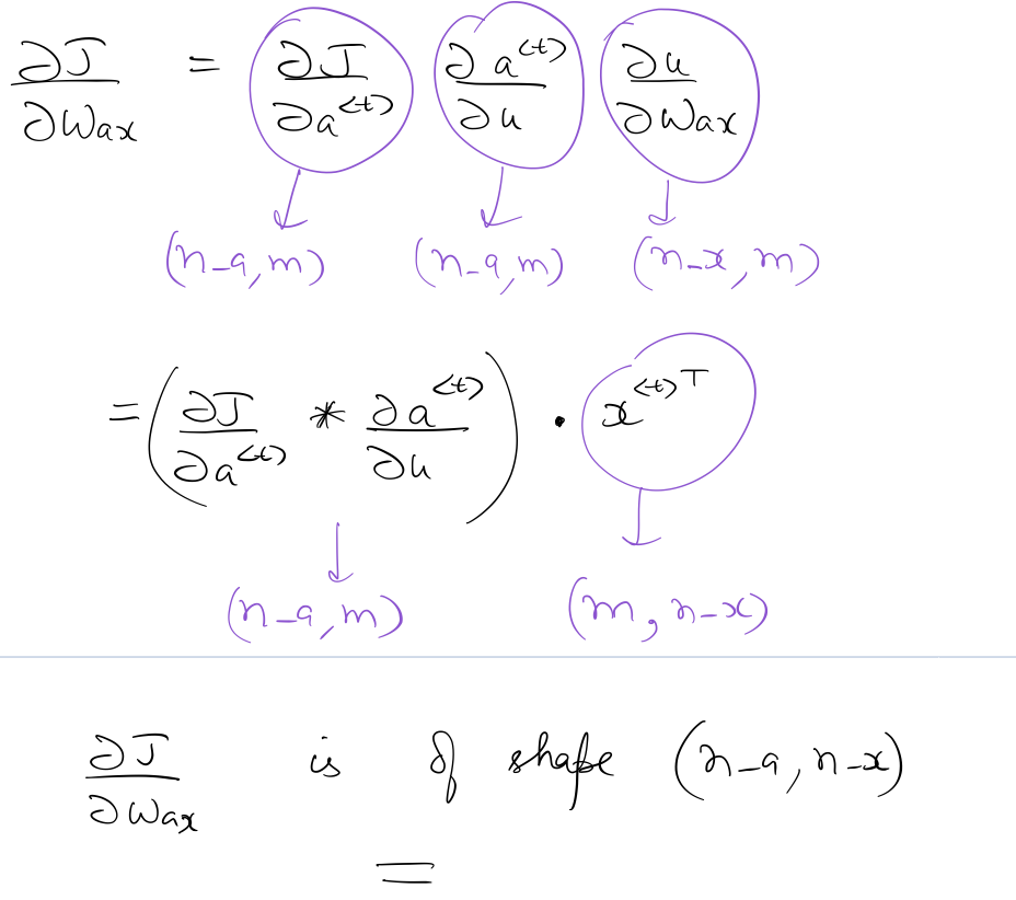
Calculation of $\frac{ \partial J } {\partial W_{ax}}$
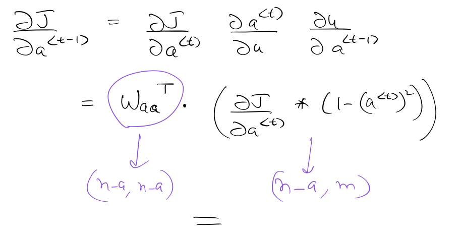
Calculation of $\frac{ \partial J } {a^{\langle t-1 \rangle}}$
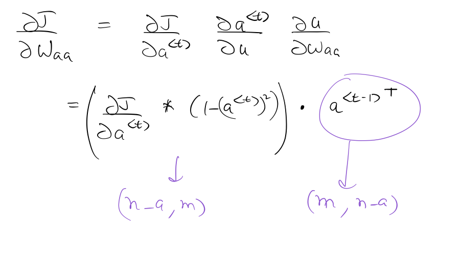
Calculation of $\frac{ \partial J } {\partial W_{aa}}$
Implementation in numpy
def rnn_step_backward(dy, gradients, parameters, x, a, a_prev):
    """
    One back propagation step for a basic RNN cell for a single time step

    Arguments:
    dy -- Gradient of Loss wrt log probabilities
    x -- input for timestep t
    a -- hidden state for time step t
    a_prev -- previous hidden state

    Returns:
    gradients -- updated gradients dictionary after performing backprop for time step t

    """
    gradients['dWya'] += np.dot(dy, a.T)
    gradients['dby'] += dy
    da = np.dot(parameters['Wya'].T, dy) + gradients['da_next']
    daraw = (1 - a * a) * da
    gradients['dba'] += daraw
    gradients['dWax'] += np.dot(daraw, x.T)
    gradients['dWaa'] += np.dot(daraw, a_prev.T)
    gradients['da_next'] = np.dot(parameters['Waa'].T, daraw)
    return gradients
def rnn_backward(X, Y, parameters, cache):
    """
    Back propagation for RNN

    Arguments:
    cache -- tuple of normalized output probabilities, a, and x

    Returns:
    updated gradients dictionary after performing backprop for all time steps
    cache -- tuple of normalized output probabilities, hidden states, and inputs for all time steps

    """

    gradients = {}

    (y_hat, a, x) = cache
    Waa, Wax, Wya, by, ba = parameters['Waa'], parameters['Wax'], parameters['Wya'],\
                            parameters['by'], parameters['ba']

    gradients['dWax'], gradients['dWaa'], gradients['dWya'] = np.zeros_like(Wax), \
                                                              np.zeros_like(Waa),\
                                                              np.zeros_like(Wya)
    gradients['dba'], gradients['dby'] = np.zeros_like(ba), np.zeros_like(by)
    gradients['da_next'] = np.zeros_like(a[0])

    # Backpropagate through time
    for t in reversed(range(len(X))):
        """
        in order to backpropagate from softmax output to class scores,
        we need to find derivative of Loss wrt class scores,
        which in case of binary outputs is simply normalized probability - 1,
        more here http://cs231n.github.io/neural-networks-case-study/#grad
        """
        dy = np.copy(y_hat[t])
        dy[Y[t]] -= 1
        gradients = rnn_step_backward(dy, gradients, parameters, x[t], a[t], a[t-1])

    return gradients, a
def update_parameters(parameters, gradients, lr):

    parameters['Wax'] -= lr * gradients['dWax']
    parameters['Waa'] -= lr * gradients['dWaa']
    parameters['Wya'] -= lr * gradients['dWya']
    parameters['ba']  -= lr * gradients['dba']
    parameters['by']  -= lr * gradients['dby']
    return parameters
Combining forward and backprop to train the model.
def train(X, Y, a_prev, parameters, learning_rate = 0.01):
    """
    One step of the optimization to train the model.

    Arguments:
    a_prev -- previous hidden state.
    learning_rate -- learning rate for the model.

    Returns:
    loss -- value of the loss function (cross-entropy)
    gradients -- python dictionary containing dWaa, dWax, dWya, dba, dby
    a[len(X)-1] -- the last hidden state, of shape (n_a, 1)
    """

    # Forward prop
    loss, cache = rnn_forward(X, Y, a_prev, parameters, n_x=27)

    # Backprop
    gradients, a = rnn_backward(X, Y, parameters, cache)

    # Update parameters
    parameters = update_parameters(parameters, gradients, learning_rate)

    return loss, gradients, a[len(X)-1], parameters
#example
#using n_x as 27, and 100 hidden states

n_x, n_a = 27, 100

#need to initialize a_prev for timestep 0
a_prev = np.random.randn(n_a, 1)

#initializing the parameters
Wax, Waa, Wya = np.random.randn(n_a, n_x), np.random.randn(n_a, n_a), np.random.randn(n_x, n_a)
ba, by = np.random.randn(n_a, 1), np.random.randn(n_x, 1)

parameters = {"Wax": Wax, "Waa": Waa, "Wya": Wya, "ba": ba, "by": by}
Let's say we want to train the RNN to predict characters based on previously seen words. Suppose as per some numerical encoding, the word 'recurrent' translates to [17, 4, 2, 20, 17, 17, 4, 13, 19]. We can train the RNN such that when it sees the sequence of characters ['r', 'e', 'c', 'u', 'r', 'r', 'e', 'n'], it predicts the next character to be 't'.
X = [17, 4, 2, 20, 17, 17, 4, 13]
Y = [4, 2, 20, 17, 17, 4, 13, 19]

loss, gradients, a_last, parameters1 = train(X, Y, a_prev, parameters, learning_rate = 0.01)
print("Loss =", loss)
This is how the RNN can be trained on sufficiently large amount of training data.