Understanding Object Detection Part 3: Single Shot Detector
This post is third in a series on object detection. The other posts can be found here, here, and here.
This post will detail a technique for classifying and localizing multiple objects in an image using a single deep neural network. Going from single object detection to multiple object detection is a fairly hard problem, so this is going to be a long post.
The approach used below is based on learnings from fastai's Deep Learning MOOC (Part 2).
!pip install -q fastai==0.7.0 torchtext==0.2.3
!wget -qq http://pjreddie.com/media/files/VOCtrainval_06-Nov-2007.tar
!tar -xf VOCtrainval_06-Nov-2007.tar
!wget -qq https://storage.googleapis.com/coco-dataset/external/PASCAL_VOC.zip
!unzip -q PASCAL_VOC.zip
!mkdir -p data/pascal
!mv PASCAL_VOC/* data/pascal
!mv VOCdevkit data/pascal
%matplotlib inline
%reload_ext autoreload
%autoreload 2
from fastai.conv_learner import *
from fastai.dataset import *

import json, pdb
from PIL import ImageDraw, ImageFont
from matplotlib import patches, patheffects
Copying the necessary functions from the last two exercises.
PATH = Path('data/pascal')
trn_j = json.load((PATH / 'pascal_train2007.json').open())
IMAGES,ANNOTATIONS,CATEGORIES = ['images', 'annotations', 'categories']
FILE_NAME,ID,IMG_ID,CAT_ID,BBOX = 'file_name','id','image_id','category_id','bbox'

cats = dict((o[ID], o['name']) for o in trn_j[CATEGORIES])
trn_fns = dict((o[ID], o[FILE_NAME]) for o in trn_j[IMAGES])
trn_ids = [o[ID] for o in trn_j[IMAGES]]

JPEGS = 'VOCdevkit/VOC2007/JPEGImages'
IMG_PATH = PATH/JPEGS
def get_trn_anno():
    trn_anno = collections.defaultdict(lambda:[])
    for o in trn_j[ANNOTATIONS]:
        if not o['ignore']:
            bb = o[BBOX]
            bb = np.array([bb[1], bb[0], bb[3]+bb[1]-1, bb[2]+bb[0]-1])
            trn_anno[o[IMG_ID]].append((bb,o[CAT_ID]))
    return trn_anno

trn_anno = get_trn_anno()
def show_img(im, figsize=None, ax=None):
    if not ax: fig,ax = plt.subplots(figsize=figsize)
    ax.imshow(im)
    ax.set_xticks(np.linspace(0, 224, 8))
    ax.set_yticks(np.linspace(0, 224, 8))
    ax.grid()
    ax.set_yticklabels([])
    ax.set_xticklabels([])
    return ax

def draw_outline(o, lw, foreground_color='black'):
    o.set_path_effects([patheffects.Stroke(
        linewidth=lw, foreground=foreground_color), patheffects.Normal()])

def draw_rect(ax, b, color="white", foreground_color='black'):
    patch = ax.add_patch(patches.Rectangle(b[:2], *b[-2:], fill=False, edgecolor=color, lw=2))
    draw_outline(patch, 4, foreground_color)

def draw_text(ax, xy, txt, sz=14,color='white'):
    text = ax.text(*xy, txt,
        verticalalignment='top', color=color, fontsize=sz, weight='bold')
    draw_outline(text, 1)
def bb_hw(a): return np.array([a[1],a[0],a[3]-a[1]+1,a[2]-a[0]+1])

def draw_im(im, ann):
    ax = show_img(im, figsize=(10,6))
    for b,c in ann:
        b = bb_hw(b)
        draw_rect(ax, b)
        draw_text(ax, b[:2], cats[c], sz=16)

def draw_idx(i):
    im_a = trn_anno[i]
    im = open_image(IMG_PATH/trn_fns[i])
    draw_im(im, im_a)
Multi-object detection
As we did the last time, we'll define the three constituents of the model:
- Data
- Architecture
- Loss Function
Data
For single object detection we set up the dataset such that it returned y as a list of (bounding box coordinates, class). For multi-object detection, we'll use the same approach with the difference that this time there can be multiple objects for one entry in y.
!mkdir -p {PATH}/tmp
CLAS_CSV = PATH/'tmp/clas.csv'
MBB_CSV = PATH/'tmp/mbb.csv'

f_model=resnet34
sz=224
bs=64
For classification task we need to set up an array that maps image_training_id to an array of category_ids which follow a standard category-to-id mapping convention.
mc is a list with the same length as trn_ids, and contains the names of categories of all objects contained in an image.
mc = [[cats[p[1]] for p in trn_anno[o]] for o in trn_ids]
draw_idx(trn_ids[4])

mc[4]
id2cat = list(cats.values())
id2cat[:2]
cat2id is a dictionary that maps a class name to a number. This convention will be used during training as well as inference.
cat2id = {v:k for k,v in enumerate(id2cat)}
cat2id
for o in mc[:5]:
    print(o)
    print(np.array([cat2id[p] for p in o]))
mcs = np.array([np.array([cat2id[p] for p in o]) for o in mc])
val_idxs = get_cv_idxs(len(trn_fns))
((val_mcs,trn_mcs),) = split_by_idx(val_idxs, mcs)
For localization we'll map bounding box coordinates with image file name. This is same as before, with the difference that this time we'll concatenate all bounding boxes instead of choosing just the largest one.
mbb = [np.concatenate([p[0] for p in trn_anno[o]]) for o in trn_ids]
mbbs = [' '.join(str(p) for p in o) for o in mbb]

df = pd.DataFrame({'fn': [trn_fns[o] for o in trn_ids], 'bbox': mbbs}, columns=['fn','bbox'])
df.to_csv(MBB_CSV, index=False)
df.head()
Ground truth data is ready to be used as a PyTorch Dataset. We'll use the same technique of concatenating the two datasets as before.
aug_tfms = [RandomRotate(3, p=0.5, tfm_y=TfmType.COORD),
            RandomLighting(0.05, 0.05, tfm_y=TfmType.COORD),
            RandomFlip(tfm_y=TfmType.COORD)]
tfms = tfms_from_model(f_model, sz, crop_type=CropType.NO, tfm_y=TfmType.COORD, aug_tfms=aug_tfms)
md = ImageClassifierData.from_csv(PATH, JPEGS, MBB_CSV, tfms=tfms, bs=bs,val_idxs=val_idxs, continuous=True, num_workers=4)
class ConcatLblDataset(Dataset):
    def __init__(self, ds, y2):
        self.ds,self.y2 = ds,y2
        self.sz = ds.sz
    def __len__(self): return len(self.ds)

    def __getitem__(self, i):
        x,y = self.ds[i]
        return (x, (y,self.y2[i]))
trn_ds2 = ConcatLblDataset(md.trn_ds, trn_mcs)
val_ds2 = ConcatLblDataset(md.val_ds, val_mcs)
md.trn_dl.dataset = trn_ds2
md.val_dl.dataset = val_ds2
Setting up some utilities to be used for plotting different colored bounding boxes and labels.
import matplotlib.cm as cmx
import matplotlib.colors as mcolors
from cycler import cycler

def get_cmap(N):
    color_norm  = mcolors.Normalize(vmin=0, vmax=N-1)
    return cmx.ScalarMappable(norm=color_norm, cmap='Set3').to_rgba

num_colr = 12
cmap = get_cmap(num_colr)
colr_list = [cmap(float(x)) for x in range(num_colr)]
def show_ground_truth(ax, im, bbox, clas=None, prs=None, thresh=0.3, fixed_color=None):
    bb = [bb_hw(o) for o in bbox.reshape(-1,4)]
    if prs is None:  prs  = [None]*len(bb)
    if clas is None: clas = [None]*len(bb)
    ax = show_img(im, ax=ax)
    for i,(b,c,pr) in enumerate(zip(bb, clas, prs)):
        if not (b[0]==0. and b[2]==1.):
            if((b[2]>0) and (pr is None or pr > thresh)):
                if not fixed_color is None:
                    color = fixed_color
                else:
                    color = colr_list[i%num_colr]
                draw_rect(ax, b, color=color)
                txt = f'{i}: '
                if c is not None: txt += ('bg' if c==len(id2cat) else id2cat[c])
                if pr is not None: txt += f' {pr:.2f}'
                draw_text(ax, b[:2], txt, color=color)
    return ax
def show_training_batch(batch_num):
trn_iter = iter(md.trn_dl)
for i in range(batch_num):
next(trn_iter)
x,y=to_np(next(iter(md.trn_dl)))
x=md.trn_ds.ds.denorm(x)
fig, axes = plt.subplots(3, 3, figsize=(9, 9))
for i,ax in enumerate(axes.flat):
show_ground_truth(ax, x[i], y[0][i], y[1][i])
plt.tight_layout()
fig_name = f'training-batch-{batch_num}.png'
plt.savefig(fig_name)
print(f'')
plt.close(fig)
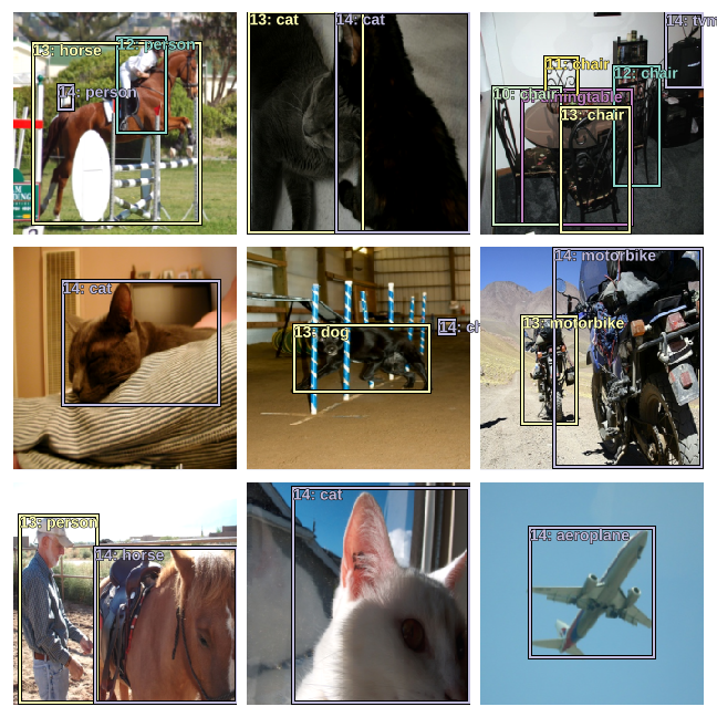
Let's take a look at the training data.
show_training_batch(0)
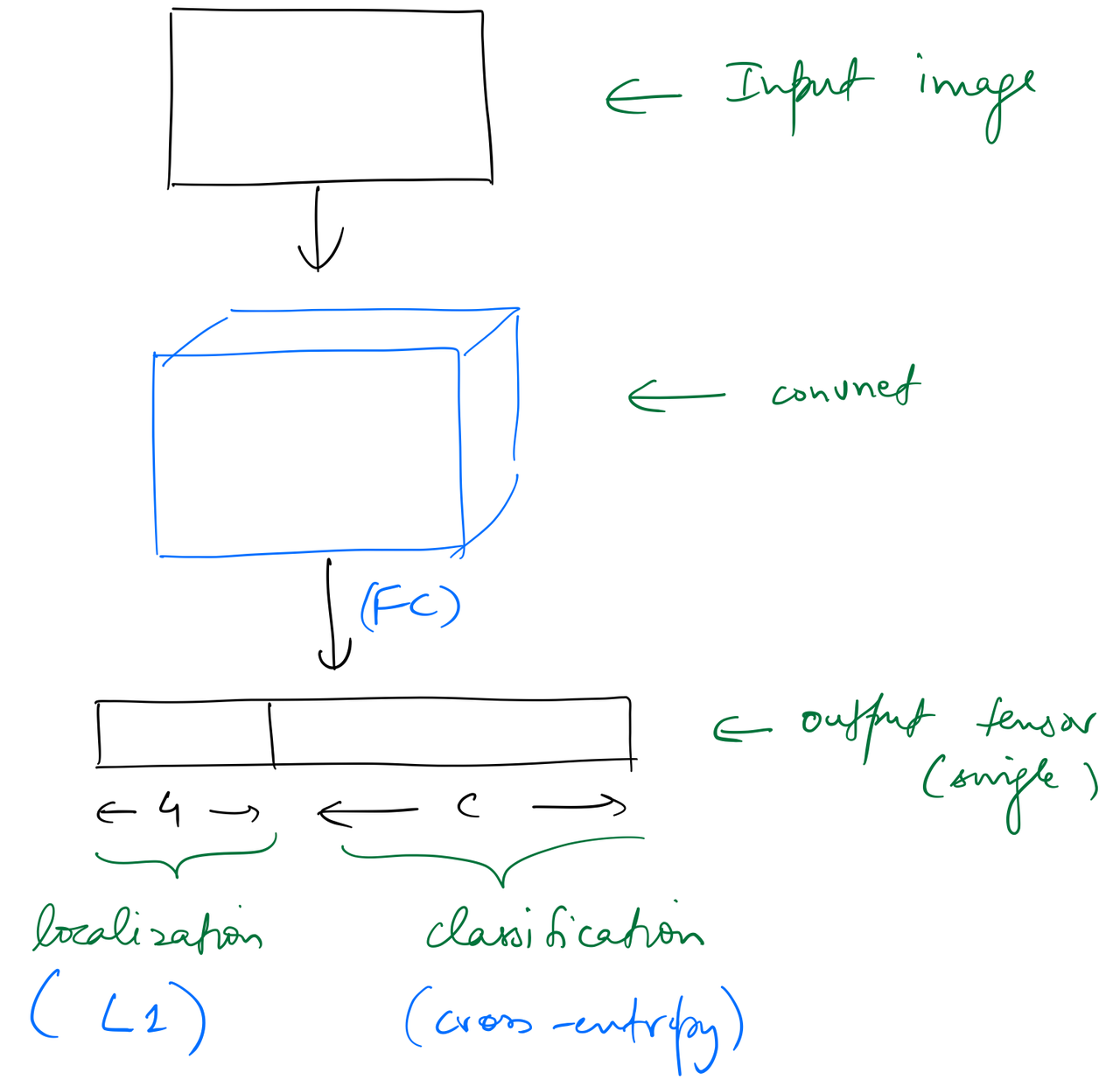
Architecture
Let’s take a look at the output activations of the network used to classify and localise one object in an image. The network outputs a tensor of shape (batch_size, (4+c)), where c is the number of categories.
This kind of architecture can be extended to identify multiple objects, say 16, by simply having a set of 16 different output activations as before, ie, having an output tensor of shape (batch_size, 16, (4+c)). Obviously, we would need a loss function that would appropriately map these 16 (4+c) activations to the ground truth, but assuming we do, this approach would work.
Another way to solve this problem would be to replace the linear layers in the custom head with a bunch of convolutional layers. Taking the example of 16 target objects as before, we can have a Conv2d layer with a stride 2, and (4+c) filters, as the custom head, which will convert the output tensor of the backbone (having shape (batch_size,7,7,512) in the running examples) into a tensor of shape (batch_size,4,4,(4+c).
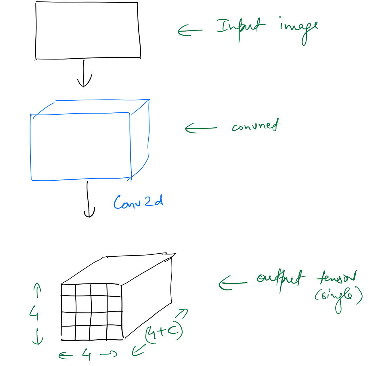
There are exactly the same number of output activations in the two approaches, but the difference between the two is that the latter retains spatial context due to the nature of the convolution operation.
I’ll focus on the second approach in this post, which is based on SSD: Single Shot MultiBox Detector by Wei Liu, Dragomir Anguelov, Dumitru Erhan, Christian Szegedy, Scott Reed, Cheng-Yang Fu, and Alexander C. Berg.
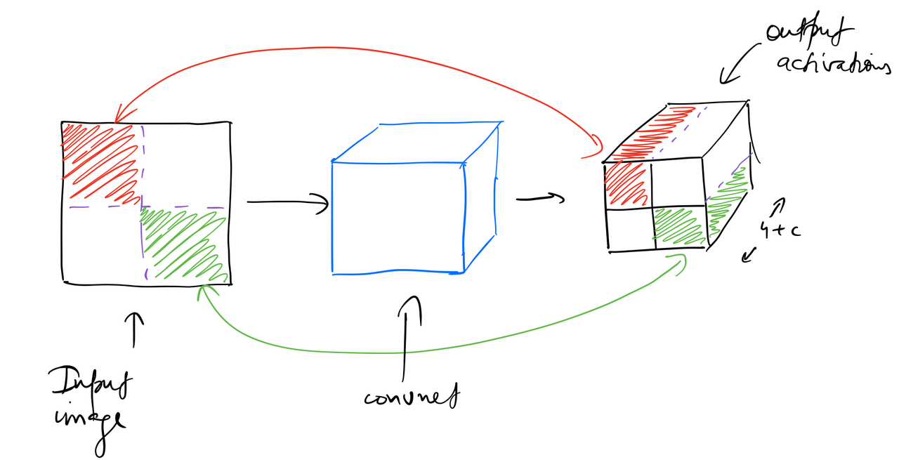
If we add another Conv2d layer to the custom head, we get a tensor of shape (batch_size,2,2,(4+c). This shape lets us map the four cells of this (2 x 2) grid to 4 quarter sub-sections of the input image by leveraging the “receptive field” of these cells.
The reason we can do this is because throughout the convolutional layers, each element of an output tensor is derived from a specific part of the input tensor, which is called it’s “receptive field”. As a result, we say that the first cell of the (2 X 2) grid should be responsible for finding an object in the top-left quarter sub-section of the input image.
Let's have a think about solving the localization problem. In the case of single-object detection, the network was outputting 4 activations for top-left and bottom-right coordinates of the bounding box, which were then being scaled to the dimensions of the input image. For multi-object detection, we'll discretize the output space of bounding boxes into a fixed grid as mentioned above. These preset boxes are also called "anchor boxes", or "default boxes". Liu et al. state in their paper:
We associate a set of default bounding boxes with each feature map cell, for multiple feature maps at the top of the network. The default boxes tile the feature map in a convolutional manner, so that the position of each box relative to its corresponding cell is fixed. At each feature map cell, we predict the offsets relative to the default box shapes in the cell, as well as the per-class scores that indicate the presence of a class instance in each of those boxes. Specifically, for each box out of
kat a given location, we computecclass scores and the4offsets relative to the original default box shape. This results in a total of(c + 4)kfilters that are applied around each location in the feature map, yielding(c + 4)kmnoutputs for am × nfeature map.
Let's set up and plot these anchor boxes. I'll use a grid size of 4 x 4, and one anchor box at a given location for now, ie, k=1.
anc_grid = 4
k = 1

anc_offset = 1/(anc_grid*2)
anc_x = np.repeat(np.linspace(anc_offset, 1-anc_offset, anc_grid), anc_grid)
anc_y = np.tile(np.linspace(anc_offset, 1-anc_offset, anc_grid), anc_grid)

anc_ctrs = np.tile(np.stack([anc_x,anc_y], axis=1), (k,1))
anc_sizes = np.array([[1/anc_grid,1/anc_grid] for i in range(anc_grid*anc_grid)])
anchors = V(np.concatenate([anc_ctrs, anc_sizes], axis=1), requires_grad=False).float()
grid_sizes = V(np.array([1/anc_grid]), requires_grad=False).unsqueeze(1)
Plotting the centers of these anchor boxes.
plt.scatter(anc_x, anc_y)
plt.xlim(0, 1)
plt.ylim(0, 1);
plt.grid(False)

We also need the corners of these anchor boxes.
def hw2corners(ctr, hw): return torch.cat([ctr-hw/2, ctr+hw/2], dim=1)
anchor_cnr = hw2corners(anchors[:,:2], anchors[:,2:])
anchor_cnr
Setting up the custom head
We know that the ResNet-34 backbone outputs a tensor of shape (batch_size,512,7,7) for this dataset. The custom head will first contain a convolutional layer with stride 1 which will only change the number of channels. Then we'll add another convolutional layer which will decrease x,y dimensions to (4,4). Till this point, classification and localization tasks share all the computation performed by the network. Let's define a module that performs all of this along with BatchNorm and non-linearity at appropriate points.
class StdConv(nn.Module):
    def __init__(self, nin, nout, stride=2, drop=0.1):
        super().__init__()
        self.conv = nn.Conv2d(nin, nout, 3, stride=stride, padding=1)
        self.bn = nn.BatchNorm2d(nout)
        self.drop = nn.Dropout(drop)

    def forward(self, x): return self.drop(self.bn(F.relu(self.conv(x))))
test = Variable(torch.randn(64,512,7,7))
s1 = StdConv(512,256, stride=1)
im1 = s1(test)
print(f'shape after 1st layer in custom head: {im1.shape}')
s2 = StdConv(256,256)
im2 = s2(im1)
print(f'shape after 2nd layer in custom head: {im2.shape}')
At this point in the network we'll split the computation for both tasks into individual convolution operations. This helps the network specialize a little bit more in each individual task.
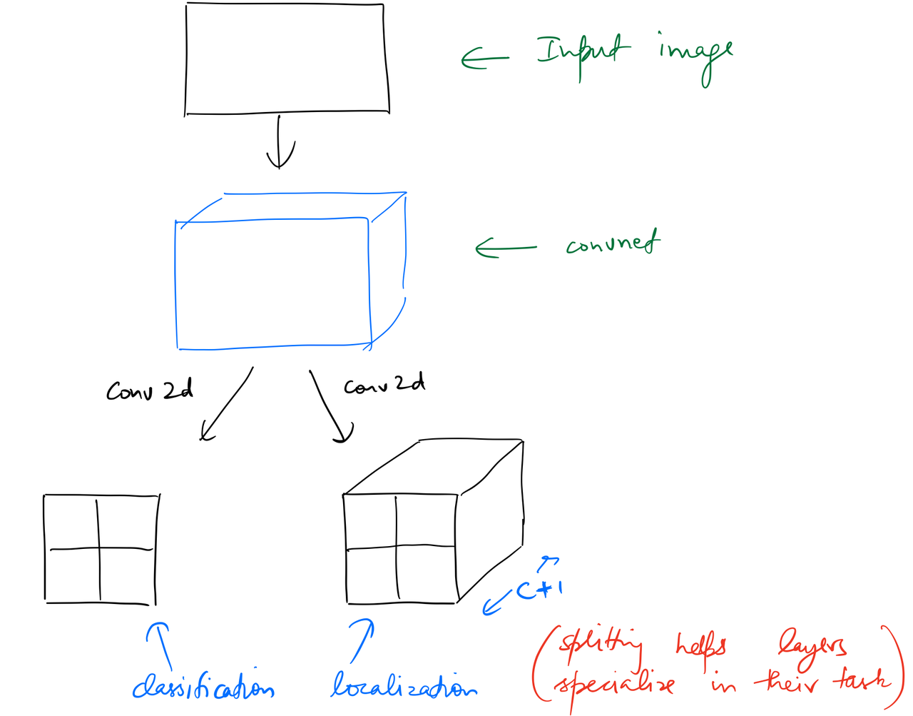
The last convolution for outputs a tensor with number_of_categories + 1 number of channels. We need to add 1 so as to predict background.
n_clas = len(id2cat)+1
n_act = k*(4+n_clas)
c1 = nn.Conv2d(256, (len(id2cat)+1)*k, 3, padding=1)(im2)
print(f'shape after last convolution for classification:\n\t{c1.shape}')
Final convolution for localization:
c2 = nn.Conv2d(256, 4*k, 3, padding=1)(im2)
print(f'shape after last convolution for localization:\n\t{c2.shape}')
We'll return a list of these two tensors after adding bias and flattening them to to get the shape (batch_size, number_of_grid_cells,necessary_activations_for_task)
def flatten_conv(x,k):
    bs,nf,gx,gy = x.size()
    x = x.permute(0,2,3,1).contiguous()
    return x.view(bs,-1,nf//k)
print(f'shape of 1st tensor of model output:\n\t{flatten_conv(c1, 1).shape}')
print(f'shape of 2nd tensor of model output:\n\t{flatten_conv(c2, 1).shape}')
Putting all of this in one module.
class OutConv(nn.Module):
    def __init__(self, k, nin, bias):
        super().__init__()
        self.k = k
        self.oconv1 = nn.Conv2d(nin, (len(id2cat)+1)*k, 3, padding=1)
        self.oconv2 = nn.Conv2d(nin, 4*k, 3, padding=1)
        self.oconv1.bias.data.zero_().add_(bias)

    def forward(self, x):
        return [flatten_conv(self.oconv1(x), self.k),
                flatten_conv(self.oconv2(x), self.k)]
o1 = OutConv(k, 256, -3.)
im3 = o1(im2)
print(im3[0].shape, im3[1].shape)
To to sum of this up, the network for multi-object detection is based on a ResNet-34 backbone and has a custom head that has convolution layera that share computation for classification and localization tasks till the second last layer, whereafter two separate convolutional layers output two separate tensors corresponding to the two tasks.
Let's define the custom head for this architecture.
class SSD_Head(nn.Module):
    def __init__(self, k, bias):
        super().__init__()
        self.drop = nn.Dropout(0.25)
        self.sconv0 = StdConv(512,256, stride=1)
        self.sconv2 = StdConv(256,256)
        self.out = OutConv(k, 256, bias)

    def forward(self, x):
        x = self.drop(F.relu(x))
        x = self.sconv0(x)
        x = self.sconv2(x)
        return self.out(x)
head_reg4 = SSD_Head(k, -3.)
models = ConvnetBuilder(f_model, 0, 0, 0, custom_head=head_reg4)
learn = ConvLearner(md, models)
learn.opt_fn = optim.Adam
Training
I'll set up the model and train it first, and then look at in detail step by step.
def one_hot_embedding(labels, num_classes):
    return torch.eye(num_classes)[labels.data.cpu()]

class BCE_Loss(nn.Module):
    def __init__(self, num_classes):
        super().__init__()
        self.num_classes = num_classes

    def forward(self, pred, targ):
        t = one_hot_embedding(targ, self.num_classes+1)
        t = V(t[:,:-1].contiguous())#.cpu()
        x = pred[:,:-1]
        w = self.get_weight(x,t)
        return F.binary_cross_entropy_with_logits(x, t, w, size_average=False)/self.num_classes

    def get_weight(self,x,t): return None

loss_f = BCE_Loss(len(id2cat))
def intersect(box_a, box_b):
    max_xy = torch.min(box_a[:, None, 2:], box_b[None, :, 2:])
    min_xy = torch.max(box_a[:, None, :2], box_b[None, :, :2])
    inter = torch.clamp((max_xy - min_xy), min=0)
    return inter[:, :, 0] * inter[:, :, 1]

def box_sz(b): return ((b[:, 2]-b[:, 0]) * (b[:, 3]-b[:, 1]))

def jaccard(box_a, box_b):
    inter = intersect(box_a, box_b)
    union = box_sz(box_a).unsqueeze(1) + box_sz(box_b).unsqueeze(0) - inter
    return inter / union
def get_y(bbox,clas):
    bbox = bbox.view(-1,4)/sz
    bb_keep = ((bbox[:,2]-bbox[:,0])>0).nonzero()[:,0]
    return bbox[bb_keep],clas[bb_keep]

def actn_to_bb(actn, anchors):
    actn_bbs = torch.tanh(actn)
    actn_centers = (actn_bbs[:,:2]/2 * grid_sizes) + anchors[:,:2]
    actn_hw = (actn_bbs[:,2:]/2+1) * anchors[:,2:]
    return hw2corners(actn_centers, actn_hw)

def map_to_ground_truth(overlaps, print_it=False):
    prior_overlap, prior_idx = overlaps.max(1)
    if print_it: print(prior_overlap)
    gt_overlap, gt_idx = overlaps.max(0)
    gt_overlap[prior_idx] = 1.99
    for i,o in enumerate(prior_idx): gt_idx[o] = i
    return gt_overlap,gt_idx

def ssd_1_loss(b_c,b_bb,bbox,clas,print_it=False):
    bbox,clas = get_y(bbox,clas)
    a_ic = actn_to_bb(b_bb, anchors)
    overlaps = jaccard(bbox.data, anchor_cnr.data)
    gt_overlap,gt_idx = map_to_ground_truth(overlaps,print_it)
    gt_clas = clas[gt_idx]
    pos = gt_overlap > 0.4
    pos_idx = torch.nonzero(pos)[:,0]
    gt_clas[1-pos] = len(id2cat)
    gt_bbox = bbox[gt_idx]
    loc_loss = ((a_ic[pos_idx] - gt_bbox[pos_idx]).abs()).mean()
    clas_loss  = loss_f(b_c, gt_clas)
    return loc_loss, clas_loss

def ssd_loss(pred,targ,print_it=False):
    lcs,lls = 0.,0.
    for b_c,b_bb,bbox,clas in zip(*pred,*targ):
        loc_loss,clas_loss = ssd_1_loss(b_c,b_bb,bbox,clas,print_it)
        lls += loc_loss
        lcs += clas_loss
    if print_it: print(f'loc: {lls.data[0]}, clas: {lcs.data[0]}')
    return lls+lcs
learn.crit = ssd_loss
lr = 3e-3
lrs = np.array([lr/100,lr/10,lr])
learn.lr_find(lrs/1000,1.)
learn.sched.plot(1)

learn.fit(lr, 1, cycle_len=5, use_clr=(20,10))
learn.save('multi')
learn.load('multi-1')
Loss Function
Loss function takes in the following two lists for one entry in the data.
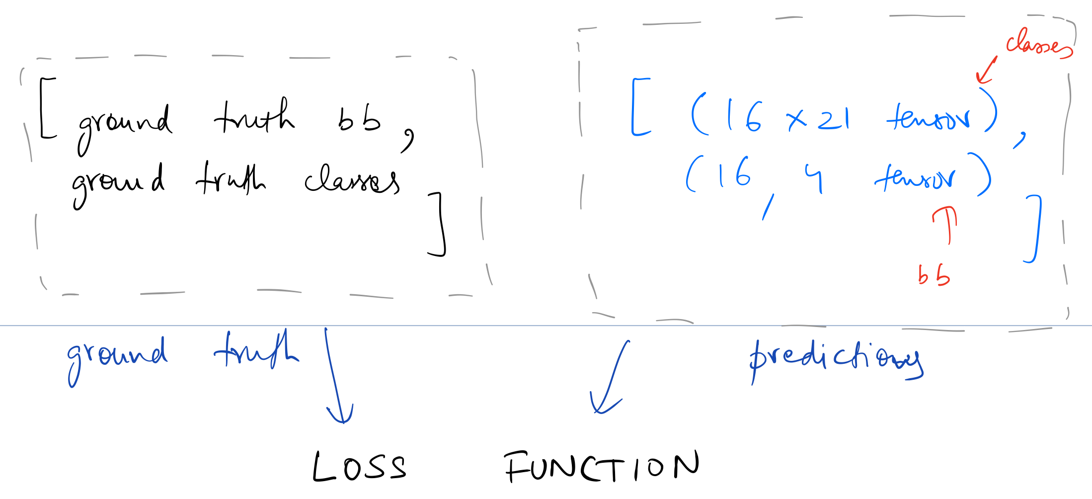
We've chosen 16 grid cells so as to be able to predict 16 unique objects in an image. The loss function needs to look at each set of 16 activations coming from the model and decide if those activations correspond to objects close or far away from the 16 grid cells, and in case no object is mapped to a grid cell, is the model predicting background. So in a way, each grid cell is responsible for coming up with a prediction of object closest to it (or else predicting background correctly)
Let's go through the logic used in calculating loss as well as the functions defined above step by step. Fetching a batch of ground truth and predictions.
itr = iter(md.val_dl)
next(itr)
x,y = next(itr)
x,y = V(x),V(y)
learn.model.eval()
batch = learn.model(x)
b_clas,b_bb = batch
y is a list of two tensors containing bounding boxes and classes respectively (both of which are zero padded by fastai by default).
y[0].shape, y[1].shape
batch is the predictions from the model, which as defined above, is a list of two flattened tensors for classification and localization respectively.
b_clas.size(),b_bb.size()
Let's stick to one image (indexed at 7 in the batch) in the validation set to better understand these variables.
-
y[0]is the ground truth bounding boxes -
y[1]is the ground truth classes
idx=10
# bounding boxes from an image in the validation set
y[0][idx][y[0][idx]>0]
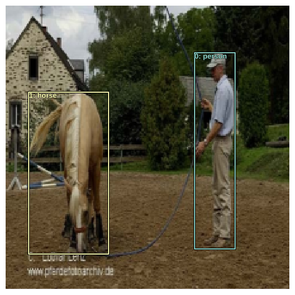
There are 2 sets of bounding boxes here, ie, 2 different objects. Let's check out the classes.
# classes from an image in the validation set
y[1][idx][y[1][idx]>0]
id2cat[14],id2cat[12]
There's a person and a horse in this image.
b_bb is the flattened tensor for bounding box prediction. Since we've specified 16 grid cells, we get 16 bounding boxes. Also, these numbers are scaled for an image of size (1 X 1).
b_bb[idx]
b_clas contains the predicted class scores for all 16 grid cells.
b_clas[idx].shape
b_clasi = b_clas[idx]
b_bboxi = b_bb[idx]
get_y (defined above) unflattens the ground truth bounding boxes tensor, scales it down to the range [0,1], and removes the zero padding done by the dataloader.
ima=md.val_ds.ds.denorm(to_np(x))[idx]
bbox,clas = get_y(y[0][idx], y[1][idx])
bbox,clas
bbox, and clas are the ground truth bounding boxes and the classes respectively. Let's see these variables plotted on the image.
def torch_gt(ax, ima, bbox, clas, prs=None, thresh=0.4, fixed_color=None):
    return show_ground_truth(ax, ima, to_np((bbox*224).long()),
         to_np(clas) if clas is not None else None, to_np(prs) if prs is not None else None, thresh, fixed_color=fixed_color)
show_ground_truth takes in numpy array of an image, along with arrays for bounding boxes, classes, and probabilities, and plots them on the image.
fig, ax = plt.subplots(figsize=(8,8))
torch_gt(ax, ima, bbox, clas);
fig_name = f'plots-1.png'
plt.savefig(fig_name)
print(f'')
plt.close(fig)
torch.cat((bbox, anchor_cnr), 0).shape
torch.cat((clas, b_clasi.max(1)[1]), 0).shape
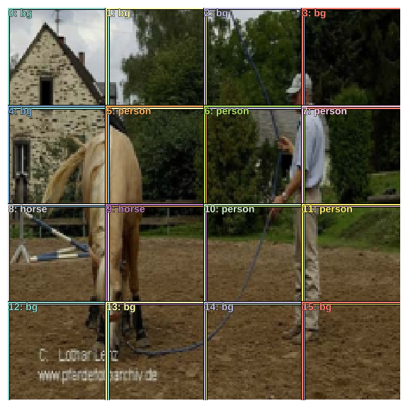
Now we'll make use of anchor corners defined above to be a set of 16 grid cells which correspond to 16 preset bounding boxes. Since the model outputs 16 set of classes we can map them one-to-one and plot them.
Note: torch.autograd.variable.Variable.max returns a tuple of tensors contains the max values and their indexes. For classes we're interested in the indexes of the max values.
anchor_cnr.shape, b_clasi.max(1)[1].shape
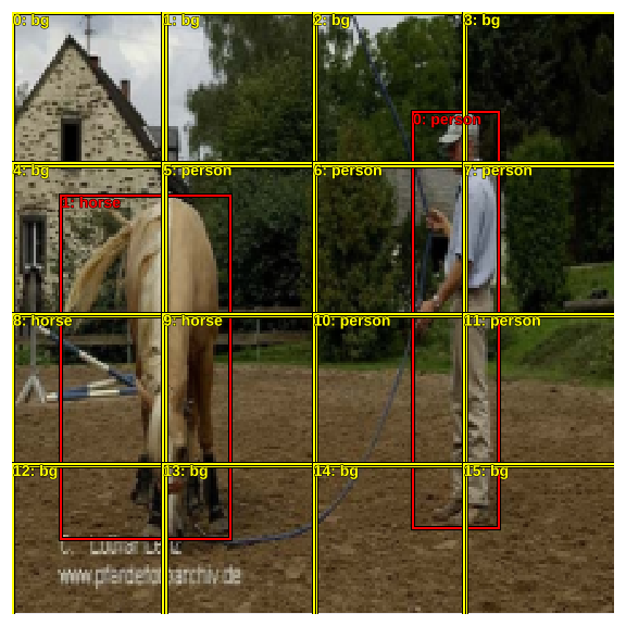
The following image shows the 16 preset anchor boxes and the predicted classes for all of them.
fig, ax = plt.subplots(figsize=(8,8))
torch_gt(ax, ima, anchor_cnr, b_clasi.max(1)[1]);
fig_name = f'plots-2.png'
plt.savefig(fig_name)
print(f'')
plt.close(fig)
Time to think about the loss function. This loss function will take the ground truth and these predicted bounding boxes and classes, and will result in a low value if these predictions are close to the ground truth.
To achieve that, we need to first "match" these anchor boxes to the ground truth. We do that by figuring out which of the anchor boxes overlap most with the ground truth bounding boxes. To do this we need to have a metric to measure the amount of overlap. We use jaccard index for this, which is the ratio area_of_intersection/area_of_union.
Liu et al. state in their paper:
During training we need to determine which default boxes correspond to a ground truth detection and train the network accordingly. For each ground truth box we are selecting from default boxes that vary over location, aspect ratio, and scale. We begin by matching each ground truth box to the default box with the best jaccard overlap. Unlike MultiBox, we then match default boxes to any ground truth with jaccard overlap higher than a threshold
(0.5). This simplifies the learning problem, allowing the network to predict high scores for multiple overlapping default boxes rather than requiring it to pick only the one with maximum overlap.
To make things easier to visualize, let's plot both the ground truth bounding boxes and the anchor boxes on the same image.
fig, ax = plt.subplots(figsize=(8,8))
ax = torch_gt(ax, ima, bbox, clas, fixed_color='red')
torch_gt(ax, ima, anchor_cnr, b_clasi.max(1)[1], fixed_color='yellow')
ax.get_xaxis().set_visible(False)
ax.get_yaxis().set_visible(False)
fig_name = f'plots-3.png'
plt.savefig(fig_name)
print(f'')
plt.close(fig)
Here we can see that ground truth bounding box for person has an overlap with 8 anchor boxes. And the ground truth bounding box for horse has an overlap with 6 anchor boxes. Let's find the jaccard index for overlap of each one of the ground-truth bounding boxes with the 16 anchor boxes.
overlaps is a (2x16) tensor containing the overlap scores for the 2 ground truth bounding boxes with the 16 anchor boxes.
overlaps = jaccard(bbox.data, anchor_cnr.data)
print('Overlap of anc boxes with gt person :')
for i,el in enumerate(overlaps[0]):
    print(f'\tanc box {i}: {el}')
print('Overlap of anc boxes with gt horse :')
for i,el in enumerate(overlaps[1]):
    print(f'\tanc box {i}: {el}')
If we find the maximum of overlaps over dimension 1, we'll get a tensor of size 2 containing the maximum value of overlap for each ground truth bounding box, as well as the indexes of the corresponding anchor boxes.
overlaps.max(1)
This means that person overlaps most with anchor box 10, and horse with anchor box 8.
We can also find out the maximum over dimension 0 which tells us the class with which each anchor box overlaps most with.
overlaps.max(0)
Now we'll use these two set of overlaps and assign each anchor box to a ground truth box using the logic stated in the SSD paper.
We'll first assign a high score to the anchor boxes with which the ground truths overlap the most. In this example it's anchor boxes 10 and 8.
gt_overlap,gt_idx = map_to_ground_truth(overlaps)
gt_overlap,gt_idx
Next we assign the anchor boxes to classes.
gt_clas = clas[gt_idx]; gt_clas
Next we match anchor boxes to any ground truth with jaccard overlap higher than a 0.5. In this example only anchor boxes 10 and 8 exceed the threshold.
thresh = 0.5
pos = gt_overlap > thresh
pos_idx = torch.nonzero(pos)[:,0]
neg_idx = torch.nonzero(1-pos)[:,0]
pos_idx
anchor_cnr[pos_idx],b_clasi.max(1)[1][pos_idx]
Now the anchor boxes selected from the above logic are assigned to their corresponding classes. The rest are assigned background.
gt_clas[1-pos] = len(id2cat); gt_clas
Let's see the classes finally assigned to each anchor box.
[id2cat[o] if o<len(id2cat) else 'bg' for o in gt_clas.data]
As expected, just two anchor boxes are assigned with objects, and the rest are background.
fig, ax = plt.subplots(figsize=(8,8))
torch_gt(ax, ima, anchor_cnr,gt_clas);
fig_name = f'plots-4.png'
plt.savefig(fig_name)
print(f'')
plt.close(fig)
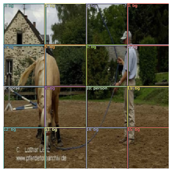
We're done with the matching problem. We've taken the ground truth and mapped it to our model's convention of 16 anchor boxes, with two anchor boxes mapped to objects and the rest being background.
Let's also plot the predicted bounding boxes. To do that we need to understand how to interpret the activations coming from the network. Liu et al. call these activations "box offsets" in the paper. This idea is to modify the shape of the anchor boxes as per the activations coming from the network so as to closely resemble the ground truth bounding boxes. This is done by actn_to_bb, which is defined as:
def actn_to_bb(actn, anchors):
    actn_bbs = torch.tanh(actn)
    actn_centers = (actn_bbs[:,:2]/2 * grid_sizes) + anchors[:,:2]
    actn_hw = (actn_bbs[:,2:]/2+1) * anchors[:,2:]
    return hw2corners(actn_centers, actn_hw)
It takes these activations of shape (16,4) and does the following:
- It passes the activations through a
tanh, which forces them to be in the range(-1,1) - It modifies the center and height-width of the anchor boxes according to the values of the activations resulting in predicted bounding boxes.
Let's take a look at the resulting bounding boxes for the example image. We also pass the class score probabilites to torch_gt to plot them.
a_ic = actn_to_bb(b_bboxi, anchors)
fig, ax = plt.subplots(figsize=(8,8))
torch_gt(ax, ima, a_ic, b_clasi.max(1)[1], b_clasi.max(1)[0].sigmoid(), thresh=0.0);
fig_name = f'plots-5.png'
plt.savefig(fig_name)
print(f'')
plt.close(fig)
It's looks quite messy but is exactly what we expected it to be. We've got 16 predicted bounding boxes, and as we can see in the image above we have multiple bounding boxes predicting the location of the same object.
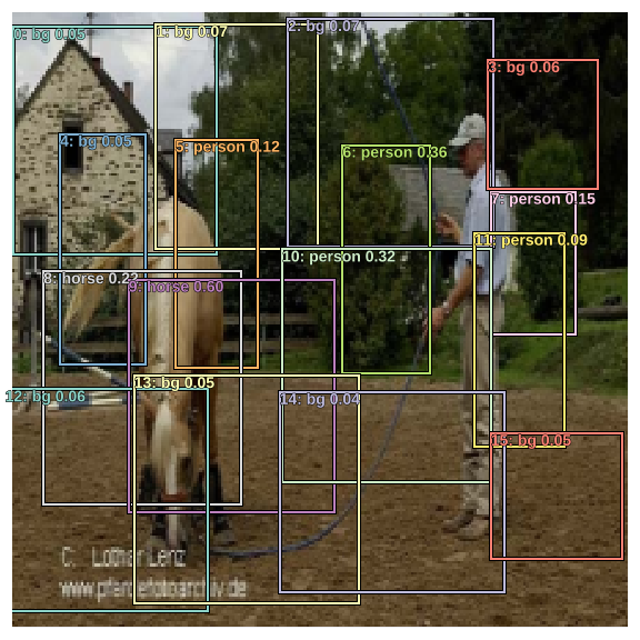
Let's take a look at the predicted bounding boxes for all objects except background.
not_bg = (b_clasi.max(1)[1]!=len(id2cat)).nonzero().view(-1)
fig, ax = plt.subplots(figsize=(8,8))
torch_gt(ax, ima, a_ic[not_bg], b_clasi.max(1)[1][not_bg], b_clasi.max(1)[0][not_bg].sigmoid(), thresh=0.0);
fig_name = f'plots-6.png'
plt.savefig(fig_name)
print(f'')
plt.close(fig)
Most predicted bounding boxes are covering only a part of the target object. This is due to the fact that the anchor boxes were small to begin with, as well as square in shape. The activations coming from the network can only increase or decrease the dimensions of these anchor boxes by 50% (refer to actn_to_bb) so that makes sense.
Localization Loss
For localization loss, we need to find L1 loss between the ground truth and predicted bounding boxes associated with the "matched" anchor boxes, ie, corresponding to pos_idx. We ignore all other predicted bounded boxes.
gt_bbox = bbox[gt_idx]
gt_bbox[pos_idx],a_ic[pos_idx]
Let's plot the bounding boxes which are used in calculating L1 loss. white is ground truth, and orange is the predictions.
fig, ax = plt.subplots(figsize=(8,8))
ax = torch_gt(ax, ima, gt_bbox[pos_idx], None, fixed_color="white") #gt
ax = torch_gt(ax, ima, a_ic[pos_idx], None, fixed_color="orange") # predictions
ax.get_xaxis().set_visible(False)
ax.get_yaxis().set_visible(False)
ax.set_title("white: GT | orange: Predictions")
fig_name = f'plots-7.png'
plt.savefig(fig_name)
print(f'')
plt.close(fig)
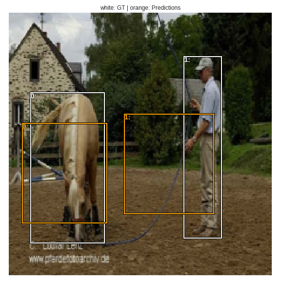
Localization loss is calculated between the white bounding boxes (ground truth) and the orange bounding boxes (predictions).
loc_loss = ((a_ic[pos_idx] - gt_bbox[pos_idx]).abs()).mean()
Classification loss
Classification loss can be calculated as cross-entropy between classes predicted and ground truth classes (after matching).
fig, ax = plt.subplots(1,2,figsize=(12,6))
ax1 = torch_gt(ax[0], ima, anchor_cnr, b_clasi.max(1)[1]);
ax1.set_title('Predictions');
ax2 = torch_gt(ax[1], ima, anchor_cnr, gt_clas);
ax2.set_title('Ground Truth');
fig_name = f'plots-8.png'
plt.savefig(fig_name)
print(f'')
plt.close(fig)
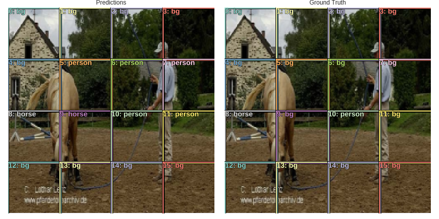
clas_loss = F.cross_entropy(b_clasi, gt_clas)
Let's check out the predictions on validation data.
def show_validation_batch(batch_num, show_bg=False, thresh=0.01, fname="1"):
val_iter = iter(md.val_dl)
for i in range(batch_num):
next(val_iter)
x,y = next(val_iter)
fig, axes = plt.subplots(4, 3, figsize=(12, 16))
x,y = V(x),V(y)
learn.model.eval()
batch = learn.model(x)
b_clas,b_bb = batch
for idx,ax in enumerate(axes.flat):
b_clasi = b_clas[idx]
b_bboxi = b_bb[idx]
ima=md.val_ds.ds.denorm(to_np(x))[idx]
bbox,clas = get_y(y[0][idx], y[1][idx])
a_ic = actn_to_bb(b_bb[idx], anchors)
overlaps = jaccard(bbox.data, anchor_cnr.data)
gt_overlap,gt_idx = map_to_ground_truth(overlaps)
gt_clas = clas[gt_idx]
pos = gt_overlap > thresh
pos_idx = torch.nonzero(pos)[:,0]
gt_clas[1-pos] = len(id2cat)
not_bg = (b_clasi.max(1)[1]!=len(id2cat)).nonzero().view(-1)
if show_bg:
torch_gt(ax, ima, a_ic, b_clasi.max(1)[1], b_clasi.max(1)[0].sigmoid(), thresh=thresh);
else:
torch_gt(ax, ima, a_ic[not_bg], b_clasi.max(1)[1][not_bg], b_clasi.max(1)[0][not_bg].sigmoid(), thresh=thresh);
plt.tight_layout()
fig_name = f'validation-batch-{fname}.png'
plt.savefig(fig_name)
print(f'')
plt.close(fig)
show_validation_batch(1, show_bg=True, fname="1")
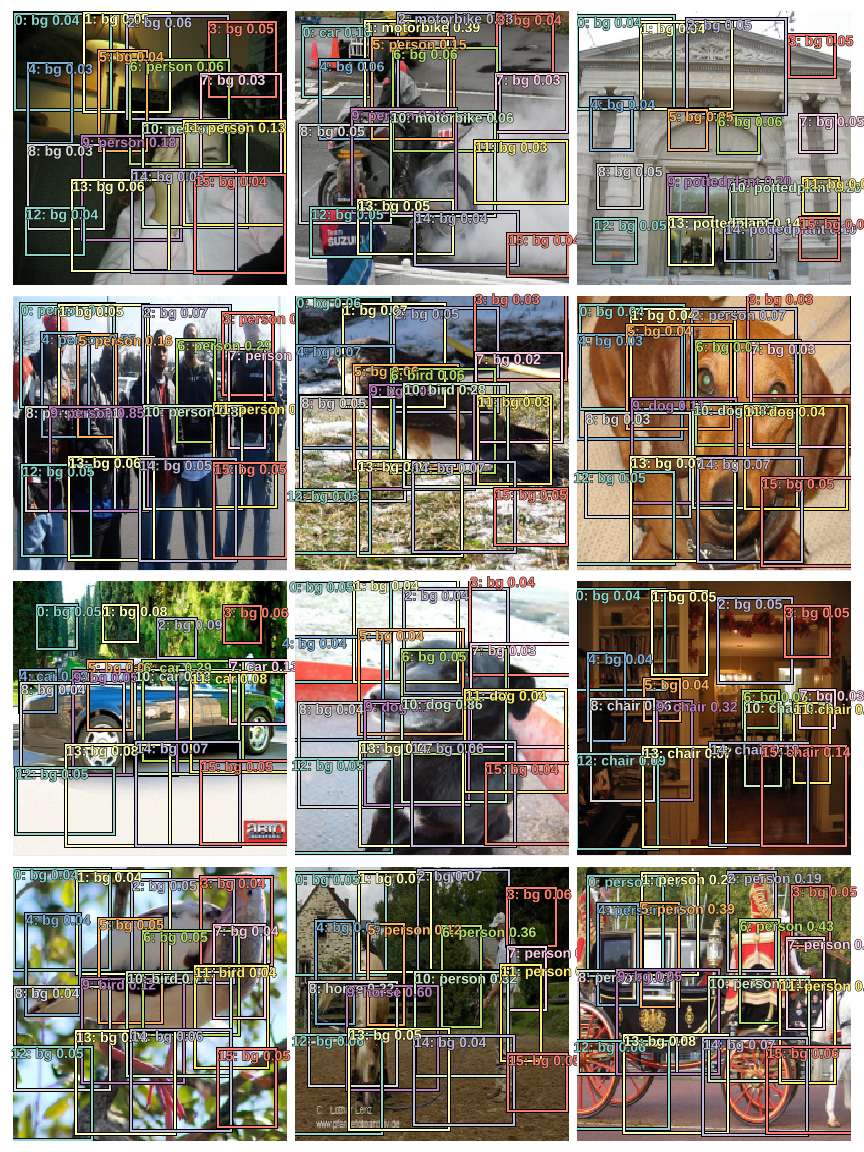
Since plotting bounding boxes for background doesn't make sense, let's skip those. We can also increase thresh so as to see skip bounding boxes for which class probabilites are very low.
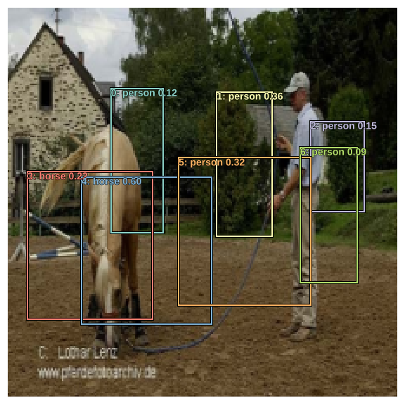
show_validation_batch(1, thresh=0.2, fname="2")
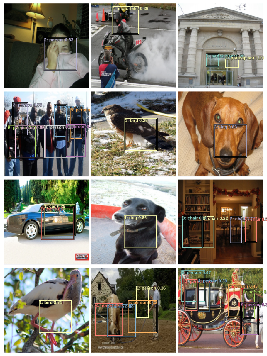
show_validation_batch(2, thresh=0.1, fname="3")
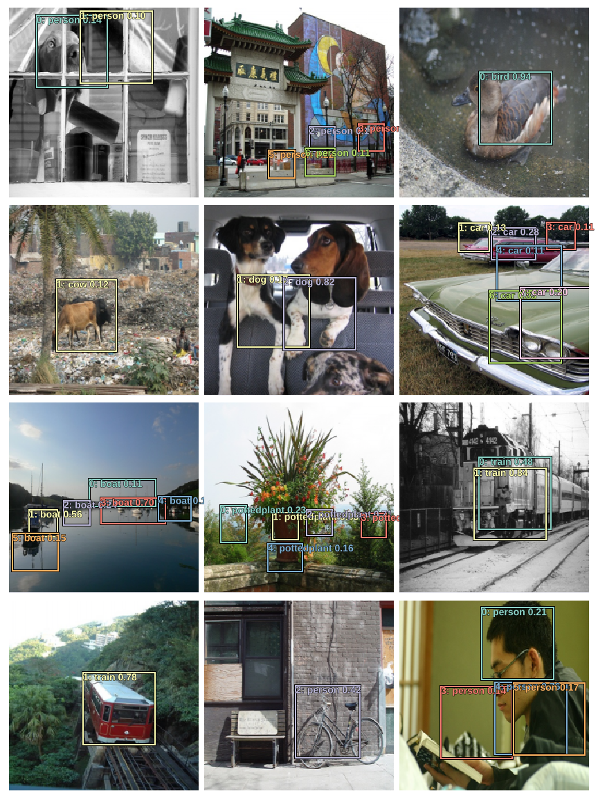
The model is able to predict multiple objects! Although, it's not doing great in the localization task, but that's due to the fact that the square and small anchor boxes chosen above only allow objects of certain shapes to be localized well. Also, the model is predicting multiple bounding boxes for the same object as evident in the above images.
The SSD paper details various ways to deal with these problems. I'll describe them in upcoming posts.
fin.