Generating artistic images using Neural Style Transfer
One of the best (and fun) ways to learn about the inner workings of convnets is through the application of Neural Style Transfer. By making use of this technique we can generate artistic versions of ordinary images in the style of a painting. NST was devised by Leon A. Gatys, Alexander S. Ecker, and Matthias Bethge and is described in their paper A Neural Algorithm of Artistic Style.
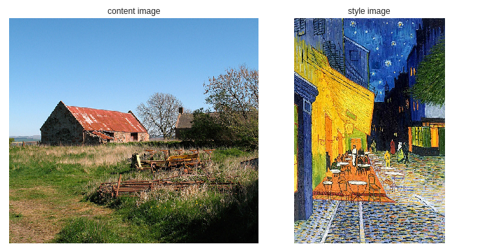
My primary motive behind this exercise is to understand how Gatys et al. used intermediate feature map activations in a convnet to generate artistic images of high perceptual quality. In order to do so, Gatys et al. define two aspects of an image: it's content and style. Content of an image refers to the objects in that image and their arrangement, whereas style refers to it's general appearance in terms of colour and textures. I’ll be using the following two images in this exercise. The first is an image of a farm which I'll refer to as the content image, and the second is Café Terrace at Night by Vincent van Gogh which I'll refer to as the style image.
%matplotlib inline
%reload_ext autoreload
%autoreload 2
!pip install -q fastai==0.7.0 torchtext==0.2.3
!apt install -q imagemagick
from fastai.conv_learner import *
from pathlib import Path
from scipy import ndimage
from math import ceil
from decimal import Decimal
from matplotlib import animation, rc
from IPython.display import HTML
PATH = Path('data/imagenet')
PATH_IMAGES = PATH/'images'
PATH_STYLE = PATH/'style'

!mkdir -p {PATH_IMAGES}
!mkdir -p {PATH_STYLE}

!wget -qq http://farm1.static.flickr.com/202/480492895_711231246a.jpg -O {PATH_IMAGES}/farm.jpg
content_img = open_image(PATH_IMAGES/'farm.jpg')

!wget -qq https://media.overstockart.com/optimized/cache/data/product_images/VG1540-1000x1000.jpg -O {PATH_STYLE}/'cafe_terrace.jpg'
style_img = open_image(PATH_STYLE/'cafe_terrace.jpg')

images = [content_img,style_img]
titles = ['content image', 'style image']

fig,axes = plt.subplots(1,2,figsize=(10,5))
for i,ax in enumerate(axes.flat):
    ax.grid(False)
    ax.get_xaxis().set_visible(False)
    ax.get_yaxis().set_visible(False)
    ax.set_title(titles[i])
    ax.imshow(images[i]);
plt.tight_layout()
plt.show()
We need a loss function that results in a lower value if the generated image matches the content of the first image, and is drawn in the style of the "Cafe Terrace at Night" painting.
Let's think about ways to find similarities between the content/style of two images.
Content similarity
We can leverage intermediate feature maps of a trained convnet for this task. If two images result in similar feature maps at a particular layer, they must be similar in terms of content.
Gatys et al. state in their paper:
When Convolutional Neural Networks are trained on object recognition, they develop a representation of the image that makes object information increasingly explicit along the processing hierarchy. Therefore, along the processing hierarchy of the network, the input image is transformed into representations that increasingly care about the actual content of the image compared to its detailed pixel values. We can directly visualise the information each layer contains about the input image by reconstructing the image only from the feature maps in that layer.
Lower layers are more closer to the input pixel values, so the feature maps from these layers closely resemble the input image. Whereas, the higher layers in the network capture high-level content in terms of objects and their arrangement. We can visualise the information each layer contains by reconstructing an image from the feature maps in that layer.
Style similarity
To obtain a representation of the style of an input image, we use a feature space originally designed to capture texture information. This feature space is built on top of the filter responses in each layer of the network. It consists of the correlations between the different filter responses over the spatial extent of the feature maps. By including the feature correlations of multiple layers, we obtain a stationary, multi-scale representation of the input image, which captures its texture information but not the global arrangement.
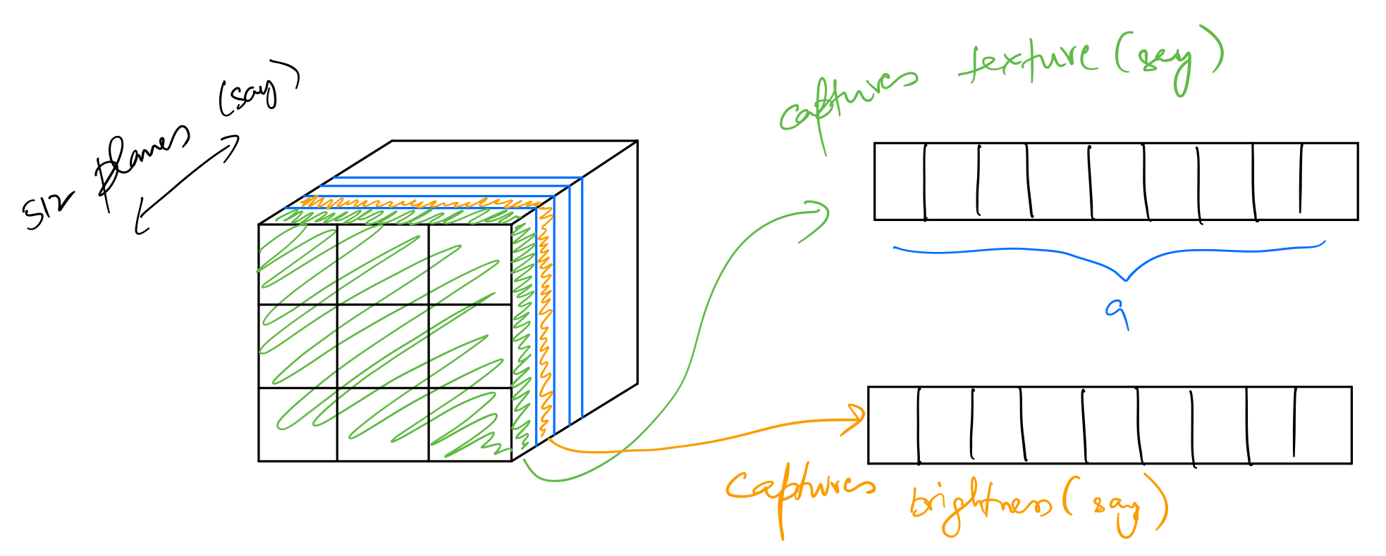
Each channel in intermediate feature activations contains information pertaining to a specific feature of the input image. Since convolution retains spatial information, each unit in a feature map corresponds to a certain region in the incoming tensor to that layer. These feature maps can capture information about different aspects of the input image, eg. texture, brightness, brush strokes, etc. Gatys et al. present a way to leverage this information captured to extract the "style" of an image. Let's see how.
Process
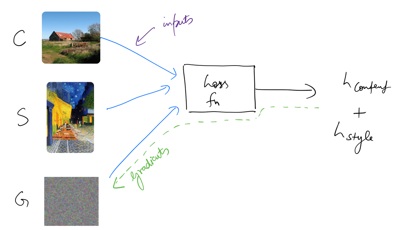
- Start with an image with random noise. Let’s call it $G$. The loss function will optimise the values of this image tensor.
- Choose intermediate layers to extract activations from. Set up hooks for these layers.
- Pass the content image through the network. Let’s call it $C$. Capture the feature map activations from the chosen intermediate layers.
- Pass the style image through the network. Let’s call it $S$. Capture the feature map activations from the chosen intermediate layers.
- In each training iteration, pass $G$ through the network. Capture the feature map activations from the chosen intermediate layers.
- Define a loss function that calculates
content_lossbetween activations from $C$ and $G$, andstyle_lossbetween activations from $S$ and $G$. The total loss will be: $$\mathcal{L}_{total}(C,S,G) = \alpha\mathcal{L}_{content}(C,G)+\beta\mathcal{L}_{style}(S,G)$$ where $\alpha$ and $\beta$ are weighting factors for content and style reconstruction respectively. - Minimise the loss using backpropagation. This will update the pixel values of $G$.
I'll use a pre-trained VGG16 (trained on imagenet) as the convnet. For NST we don't need to update the parameters of the network itself.
m_vgg = to_gpu(vgg16(True)).eval()
set_trainable(m_vgg, False)
sz=288
trn_tfms,val_tfms = tfms_from_model(vgg16, sz)
img_tfm = val_tfms(content_img)
img_tfm.shape
Starting with $G$ with random noise and the same shape as content image.
opt_img = np.random.uniform(0, 1, size=content_img.shape).astype(np.float32)
opt_img = scipy.ndimage.filters.median_filter(opt_img, [10,10,1])
fig,axes = plt.subplots(1,1,figsize=(5,5))
axes.grid(False)
axes.get_xaxis().set_visible(False)
axes.get_yaxis().set_visible(False)
axes.imshow(opt_img);
plt.tight_layout()
plt.savefig('random_noise.png')

Next, let's define the intermediate layers from which to extract activations. We'll use PyTorch hooks for this.
class SaveFeatures():
    features=None
    def __init__(self, m): self.hook = m.register_forward_hook(self.hook_fn)
    def hook_fn(self, module, input, output): self.features = output
    def close(self): self.hook.remove()
Let's use the layers just before a Max-Pool for reconstruction.
block_ends = [i-1 for i,o in enumerate(children(m_vgg))
              if isinstance(o,nn.MaxPool2d)]
block_ends
Layers numbered 5, 12, 22, and 32 will be used. Let's set up a hook on layer 32.
sf = SaveFeatures(children(m_vgg)[block_ends[-1]])
Putting together a function that returns $G$ as a PyTorch variable, and an optimiser for the same.
def get_opt():
    opt_img = np.random.uniform(0, 1, size=content_img.shape).astype(np.float32)
    opt_img = scipy.ndimage.filters.median_filter(opt_img, [8,8,1])
    opt_img_v = V(val_tfms(opt_img/2)[None], requires_grad=True)
    return opt_img_v, optim.LBFGS([opt_img_v])
opt_img_v, optimizer = get_opt()
As mentioned in the process above, we need to run a forward pass for $G$, $C$, and $S$ through the network.
m_vgg(opt_img_v)
intermediate_G_activations = V(sf.features.clone())
intermediate_G_activations.shape
img_tfm = val_tfms(content_img)
m_vgg(VV(img_tfm[None]))
intermediate_C_activations = V(sf.features.clone())
intermediate_C_activations.shape
style_tfm = val_tfms(style_img)
m_vgg(VV(style_tfm[None]))
intermediate_S_activations = V(sf.features.clone())
intermediate_S_activations.shape
Layer 32 outputs activation tensor of shape (batch_size,512,18,18). Calculating content_loss is pretty straightforward. We calculate mse loss between activations from $C$ and those from $G$.
content_loss = F.mse_loss(intermediate_C_activations, intermediate_G_activations)
content_loss.data
Gram Matrix
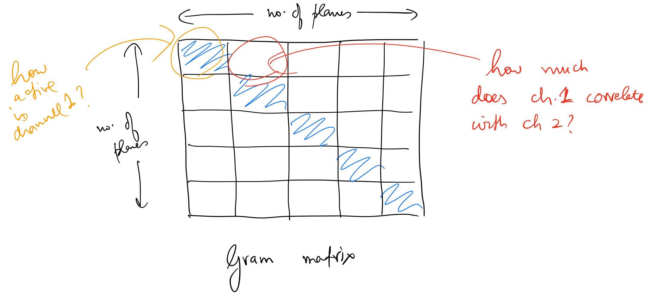
To calculate style_loss we need to represent the correlations between different channels in the activations tensor. We do this by generating a gram matrix from the activations tensor. First, we expand the activations tensor along height and width dimensions. For example, a (512,18,18) tensor will be converted into a matrix of shape (512,18*18). Then, we'll calculate a matrix product of this matrix with itself. This will result in a (512,512) matrix where each element corresponds to correlation between two channels.
Each channel captures information corresponding to some specific feature in the input image. This is then converted into a gram matrix shown below.
tt = Variable(torch.randn(1,512,18,18))
b,c,h,w = tt.size()
tt1 = tt.view(b*c, -1)
print(tt1.shape)
print((torch.mm(tt1, tt1.t())/tt.numel()).shape)
Gram matrix gives us a measure for two things:
- The diagonal of this matrix represents correlation of all channels with themselves. This is a measure of how active a particular channel is.
- Other elements represent correlation of two separate channels. If the value of one of these elements is high, this means features corresponding to those two channels show up together in the input image.
Finally, we calculate mse loss between gram matrices generated from $G$ and $S$. This is how the "style" of the style image is replicated. Backpropagation will result in a $G$ that yields a gram matrix similar to that of $S$.
Putting this in separate functions.
def gram(input):
        b,c,h,w = input.size()
        x = input.view(b*c, -1)
        return torch.mm(x, x.t())/input.numel()*1e6

def gram_mse_loss(input, target): return F.mse_loss(gram(input), gram(target))
style_loss = gram_mse_loss(intermediate_G_activations, intermediate_S_activations)
style_loss.data
As seen above, magnitudes of content_loss and style_loss lie at different scales. The final loss value will depend on values of weighting factors $\alpha$ and $\beta$ .
Putting all of this in a single class.
class NeuralStyleTransfer(object):

    def __init__(self,base_model,sz):
        self.base_model = base_model
        self.sz = sz
        self.model = to_gpu(base_model(True)).eval()
        set_trainable(self.model, False)
        self.trn_tfms,self.val_tfms = tfms_from_model(self.base_model, self.sz)

    def get_opt(self,img):
        opt_img = np.random.uniform(0, 1, size=img.shape).astype(np.float32)
        opt_img = scipy.ndimage.filters.median_filter(opt_img, [8,8,1])
        opt_img_v = V(self.val_tfms(opt_img/2)[None], requires_grad=True)
        return opt_img_v, optim.LBFGS([opt_img_v])

    def step(self,loss_fn):
        self.optimizer.zero_grad()
        loss = loss_fn(self.opt_img_v)
        loss.backward()
        self.n_iter+=1
#         if self.print_losses:
#             if self.n_iter%self.show_iter==0: print(f'Iteration: {self.n_iter}, loss: {loss.data[0]}')
        return loss

    def scale_match(self, src, targ):
        h,w,_ = src.shape
        sh,sw,_ = targ.shape
        rat = max(h/sh,w/sw); rat
        res = cv2.resize(targ, (int(sw*rat), int(sh*rat)))
        return res[:h,:w]

    def gram(self,input):
        b,c,h,w = input.size()
        x = input.view(b*c, -1)
        return torch.mm(x, x.t())/input.numel()*1e6

    def gram_mse_loss(self,input, target):
        return F.mse_loss(self.gram(input), self.gram(target))

    def comb_loss(self,x):
        self.model(self.opt_img_v)
        content_outs = [V(o.features) for o in self.content_sfs]
        style_outs = [V(o.features) for o in self.style_sfs]

#         content_loss
        content_losses   = [F.mse_loss(o, s)
                        for o,s in zip(content_outs, self.targ_vs)]

#         style_loss
        style_losses = [self.gram_mse_loss(o, s)
                        for o,s in zip(style_outs, self.targ_styles)]


        if self.content_layers_weights is None:
            content_loss = sum(content_losses)
        else:
            content_loss = sum([a*b for a,b in
                                zip(content_losses,self.content_layers_weights)])

        if self.style_layers_weights is None:
            style_loss = sum(style_losses)
        else:
            style_loss = sum([a*b for a,b in
                              zip(style_losses,self.style_layers_weights)])
        if self.print_losses:
            if self.n_iter%self.show_iter==0:
                print(f'content: {self.alpha*content_loss.data[0]}, style: {self.beta*style_loss.data[0]}')

        if self.return_intermediates and self.n_iter<=self.gif_iter_till:
            if self.n_iter%self.gif_iter==0:
                self.intermediate_images.append(self.val_tfms.denorm(np.rollaxis(to_np(self.opt_img_v.data),1,4))[0])

        return self.alpha*content_loss + self.beta*style_loss

    def generate(self, content_image, style_img,
                 style_layers, content_layers,
                 alpha=1e6,
                 beta=1.,
                 content_layers_weights=None,
                 style_layers_weights=None,
                 max_iter=500,show_iter=300,
                 print_losses=False,
                 scale_style_img=True,
                 return_intermediates=False,
                 gif_iter=50,
                 gif_iter_till=500):

        self.max_iter = max_iter
        self.show_iter = show_iter
        self.gif_iter = gif_iter
        self.gif_iter_till = gif_iter_till

        self.alpha = alpha
        self.beta = beta
        self.content_layers_weights = content_layers_weights
        self.style_layers_weights = style_layers_weights
        self.print_losses = print_losses
        self.return_intermediates = return_intermediates
        self.intermediate_images = []

        self.content_sfs = [SaveFeatures(children(self.model)[idx]) for idx in content_layers]

        self.style_sfs = [SaveFeatures(children(self.model)[idx]) for idx in style_layers]

#         get target content
        img_tfm = self.val_tfms(content_image)
        self.opt_img_v, self.optimizer = self.get_opt(content_image)
        self.model(VV(img_tfm[None]))
        self.targ_vs = [V(o.features.clone()) for o in self.content_sfs]

#         get target style
        if scale_style_img:
            style_img = self.scale_match(content_image, style_img)
        self.style_tfm = self.val_tfms(style_img)
        self.model(VV(self.style_tfm[None]))
        self.targ_styles = [V(o.features.clone()) for o in self.style_sfs]

        self.n_iter=0

        while self.n_iter <= self.max_iter: self.optimizer.step(partial(self.step,self.comb_loss))
        for sf in self.content_sfs: sf.close()
        for sf in self.style_sfs: sf.close()
        if not self.return_intermediates:
            return self.val_tfms.denorm(np.rollaxis(to_np(self.opt_img_v.data),1,4))[0]
        else:
            return self.intermediate_images
step function is the implementation of a training loop, and scale_match transforms the style image to match the dimensions of the content image. I'll also use activations from several intermediate layers for style loss.
Time to run some experiments.
t1 = NeuralStyleTransfer(vgg16,400)
Reconstructing content from different layers without style
Let's first see the content reconstructions from various intermediate layers in the network. $\beta$ is set to $0$.
content_layers_to_use = [2,9,16,22,26,32]

n_cols = 3
n_rows = ceil(len(content_layers_to_use)/n_cols)

fig,axes = plt.subplots(n_rows,n_cols, figsize=(n_cols*4,n_rows*4))

for i,ax in enumerate(axes.flat):
    ax.grid(False)
    ax.set_xticks([])
    ax.set_yticks([])
    if i==len(content_layers_to_use):
        break
    print(f'Reconstructing content from layer {content_layers_to_use[i]}...')


    ax.set_title(f'Layer {content_layers_to_use[i]}')
    gen4 = t2.generate(content_img, style_img,
                       content_layers=[content_layers_to_use[i]],
                       style_layers=[10],
                       alpha=1e4,
                       beta=0.,
                       max_iter=1000)
    x = np.clip(gen4, 0, 1)
    ax.imshow(x,interpolation='lanczos')
plt.tight_layout()
plt.show()
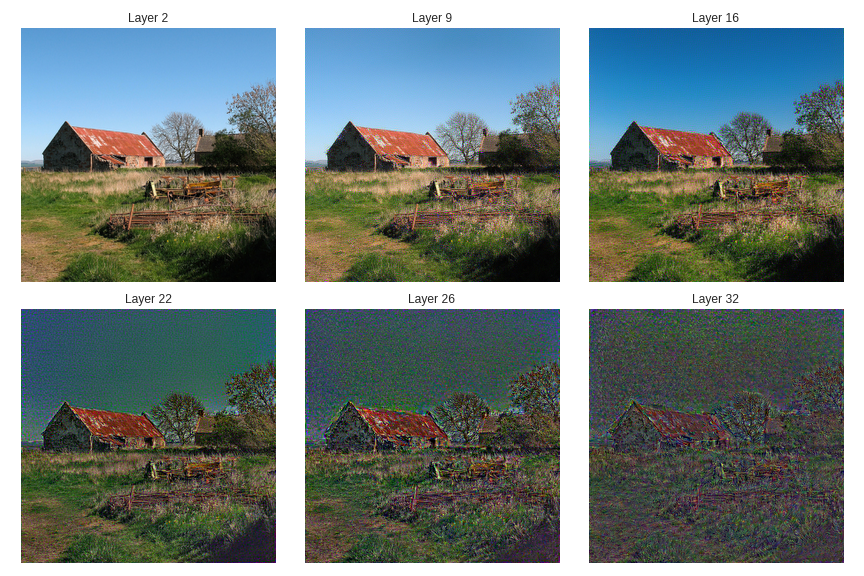
As expected, reconstructions from lower layers are much closer to the input pixel values, whereas those from higher layers capture high-level content in terms of the position and arrangement of the objects. In order to generate artistic images, layer 22 seems to be a good choice.
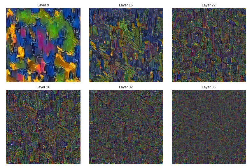
Reconstructing style from different layers without content
Let's see the style reconstructions from various intermediate layers in the network. $\alpha$ is set to $0$.
style_layers_to_use = [9,16,22,26,32,36]

n_cols = 3
n_rows = ceil(len(style_layers_to_use)/n_cols)

fig,axes = plt.subplots(n_rows,n_cols, figsize=(n_cols*4,n_rows*4))

for i,ax in enumerate(axes.flat):
    ax.grid(False)
    ax.set_xticks([])
    ax.set_yticks([])
    if i==len(style_layers_to_use):
        break
    print(f'Reconstructing style from layer {style_layers_to_use[i]}...')


    ax.set_title(f'Layer {style_layers_to_use[i]}')
    gen4 = t2.generate(content_img, style_img,
                       content_layers=[16],
                       style_layers=[style_layers_to_use[i]],
                       alpha=0.,
                       beta=1.,
                       max_iter=500)
    x = np.clip(gen4, 0, 1)
    ax.imshow(x,interpolation='lanczos')
plt.tight_layout()
plt.show()
Reconstructing style from different layers keeping content fixed
Fixing content layers to be [19,22], let's reconstruct style from a bunch of 5 layers at a time, while going deeper in the network.
style_layers_to_use = [
    [2,5,9,12,16],
    [9,12,16,22,26],
    [16,22,26,29,32],
]

n_cols = 3
n_rows = ceil(len(style_layers_to_use)/n_cols)

fig,axes = plt.subplots(n_rows,n_cols, figsize=(n_cols*4,n_rows*4))

for i,ax in enumerate(axes.flat):
    ax.grid(False)
    ax.set_xticks([])
    ax.set_yticks([])
    if i==len(style_layers_to_use):
        break
    print(f'Reconstructing style from layers {style_layers_to_use[i]}...')


    ax.set_title(f'Layer {style_layers_to_use[i]}')
    gen4 = t2.generate(content_img, style_img,
                       content_layers=[19,22],
                       style_layers=style_layers_to_use[i],
                       alpha=1e5,
                       beta=1.,
                       max_iter=800)
    x = np.clip(gen4, 0, 1)
    ax.imshow(x,interpolation='lanczos')
plt.tight_layout()
plt.show()
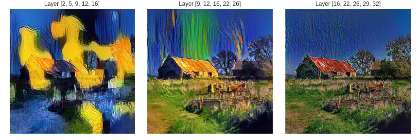
Layers [9,12,16,22,26] seem to be a good choice to reconstruct style from.
Varying $\alpha$ and $\beta$ ratios
Let's reconstruct from all chosen intermediate layers (ie, content from layer 2, style from all with equal weightage), but this time vary the ratio $\frac{\alpha}{\beta}$. We expect content of the input image to get more and more prominent as this ratio increases.
betas = [1e2,5e1,1e1,1.,5e-1,1e-1]
alpha= 1e6
ratios = ["{:.2E}".format(Decimal(alpha/b)) for b in betas]

n_cols = 3
n_rows = ceil(len(ratios)/n_cols)

fig,axes = plt.subplots(n_rows,n_cols, figsize=(n_cols*4,n_rows*4))

for i,ax in enumerate(axes.flat):
    ax.grid(False)
    ax.set_xticks([])
    ax.set_yticks([])
    if i==len(ratios):
        break
    print(f'Reconstructing with ratio {ratios[i]}...')


    ax.set_title(f'Ratio {ratios[i]}')
    gen4 = t2.generate(content_img, style_img,
                       content_layers=[19,22],
                       style_layers=[9,12,16,22,],
                       alpha=1e5,
                       beta=betas[i],
                       max_iter=1000)
    x = np.clip(gen4, 0, 1)
    ax.imshow(x,interpolation='lanczos')
plt.tight_layout()
plt.show()
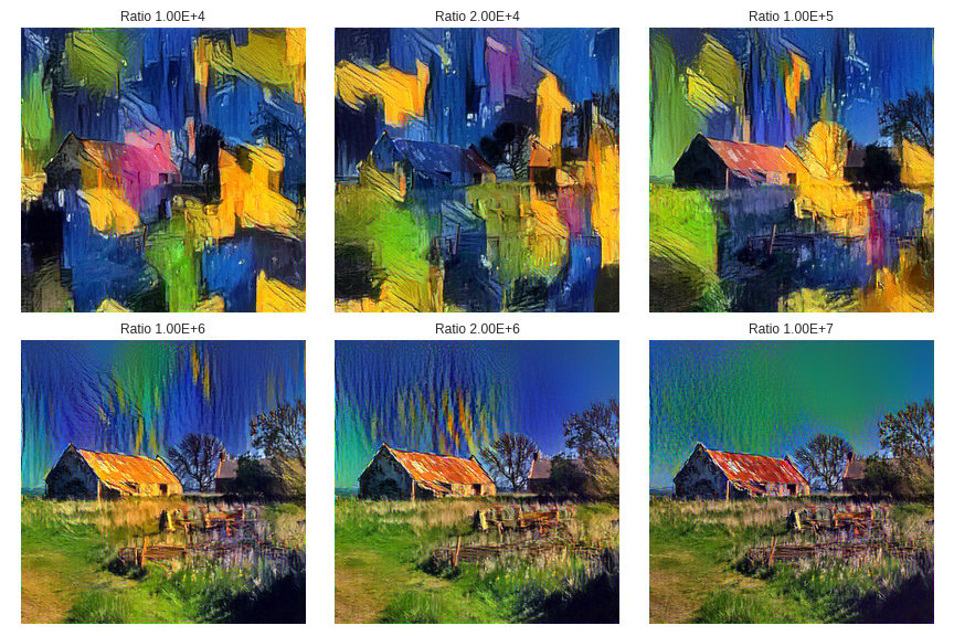
As expected, the content get more and more prominent as the ratio increases.
Visualizing updates to $G$
imgs = t2.generate(content_img, style_img,
                       content_layers=[16,22,26],
                       style_layers=[9,12,16,22,26],
                       alpha=1e5,
                       beta=1.,
                       style_layers_weights=None,
                       max_iter=800,show_iter=100,
                       print_losses=True,
                       scale_style_img=True,
                       return_intermediates=True,
                       gif_iter=50,
                       gif_iter_till=500)

fig, ax = plt.subplots(figsize=(5,5))
ax.grid(False)
ax.get_xaxis().set_visible(False)
ax.get_yaxis().set_visible(False)
fig.tight_layout()
ims = []
for i,img in enumerate(imgs):
    txt = plt.text(10,15,f'{i*50}',color='white', fontsize=16, weight='bold')
    im = ax.imshow(np.clip(img, 0, 1), interpolation='lanczos', animated=True)

    ims.append([im,txt])

ani = animation.ArtistAnimation(fig, ims, interval=300, blit=True,
                            repeat=False)
plt.close()
gif_name='style_9_12_16_22_26.gif'
ani.save(gif_name, writer='imagemagick', fps=2)
The number on each frame represents optimisation iterations. As seen above $G$ is gettting pretty good just after 4 frames, ie, 200 iterations.
Results with different style images
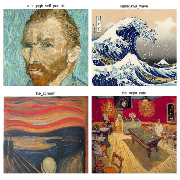
Let's plot the content picture in styles of other paintings.
paintings = {
    "van_gogh_self_portrait":"https://cdn.shopify.com/s/files/1/0223/4033/products/V495_bfc78f33-3b1a-40ec-bd64-f85c4ec05fa4_1024x1024.jpg",
    "kanagawa_wave":"https://upload.wikimedia.org/wikipedia/commons/thumb/0/0a/The_Great_Wave_off_Kanagawa.jpg/1024px-The_Great_Wave_off_Kanagawa.jpg",
    "the_scream":"https://images-na.ssl-images-amazon.com/images/I/81Z7qbHAjDL._SY679_.jpg",
    "the_night_cafe":"http://cdn.artobserved.com/2009/03/vincent-van-gogh-the-night-cafe-1888-via-artstor-collections.jpg"
}
for painting in paintings:
    print(f'!wget -qq "{paintings[painting]}" -O {PATH_STYLE}/{painting}.jpg')
    !wget -qq "{paintings[painting]}" -O {PATH_STYLE}/{painting}.jpg
style_paintings = []
paintings_names = []

for painting in paintings:
    try:
        style_paintings.append(open_image(f'{PATH_STYLE}/{painting}.jpg'))
        paintings_names.append(painting)
    except Exception as e:
        print(str(e))
n_cols = 2
n_rows = ceil(len(style_paintings)/n_cols)

fig,axes = plt.subplots(n_rows,n_cols, figsize=(n_cols*4,n_rows*4))

for i,ax in enumerate(axes.flat):

    ax.grid(False)
    ax.set_xticks([])
    ax.set_yticks([])
    ax.set_title(f'{paintings_names[i]}')
    ax.imshow(t2.scale_match(content_img, style_paintings[i]))
plt.tight_layout()
plt.show()
def show_generated_images(style_paintings,paintings_names,content_img,
                         n_cols=2,
                         alpha=1e5,
                         beta=1.):
    n_cols = n_cols
    n_rows = ceil(len(style_paintings)/n_cols)

    fig,axes = plt.subplots(n_rows,n_cols, figsize=(n_cols*4,n_rows*4))

    for i,ax in enumerate(axes.flat):
        if i==len(style_paintings):
            break

        print(f'Generating {i+1}: {paintings_names[i]}...')
        ax.grid(False)
        ax.set_xticks([])
        ax.set_yticks([])
        ax.set_title(f'{paintings_names[i]}')
        gen4 = t2.generate(content_img, style_paintings[i],
                           content_layers=[19,22],
                           style_layers=[9,12,16,22,],
                           alpha=alpha,
                           beta=beta,
                           max_iter=1000)

        x = np.clip(gen4, 0, 1)
        ax.imshow(x,interpolation='lanczos')
    plt.tight_layout()
    plt.show()
show_generated_images(style_paintings,paintings_names,content_img,beta=3.)
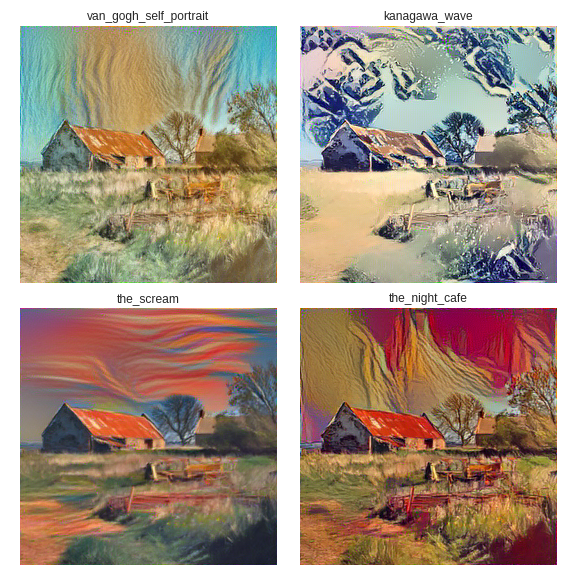
It's fascinating to see that a convnet that is trained to classify objects is able to learn image representations that allow the separation of image content from style. Gatys et al. state that the explanation for this could be that in order to get good at classifying objects, the network has to become invariant to all variations that a particular object can have in multiple images.
I'll be adding more experiments on NST here.