ML Basics #2: Multilayer Perceptron
This is the second post in this series on the basics of Machine Learning. These posts are intended to serve as companion pieces to this zine on binary classification. The last post detailed the functioning of an artificial neuron, and how it can be trained to linearly segment a dataset. However, most real world datasets are not linearly separable, which begs the question:
What is the point of learning about a neuron?
Well, by the end of this post, we'll see that a bunch of neurons, when stacked together, can learn to create powerful non-linear solution spaces. Let's see how that works.
Setup
!apt-get install imagemagick
!pip install -q celluloid
from sklearn.datasets import make_classification
import matplotlib.pyplot as plt
import numpy as np
import pandas as pd
from IPython.display import HTML
import pickle
from math import ceil
from matplotlib.offsetbox import AnchoredText
from celluloid import Camera
def plot_points(X, y, alpha=None):
    dogs = X[np.argwhere(y==1)]
    cats = X[np.argwhere(y==0)]
    plt.scatter([s[0][0] for s in cats], [s[0][1] for s in cats], s = 25, \
                color = 'red', edgecolor = 'k', label='cat', alpha=alpha)
    plt.scatter([s[0][0] for s in dogs], [s[0][1] for s in dogs], s = 25, \
                color = 'blue', edgecolor = 'k', label='dog', alpha=alpha)
    plt.xlabel('$x_1$')
    plt.ylabel('$x_2$')
    plt.legend()
This is what we've learnt so far: A neuron's weights and bias can be optimised using gradient descent to create a linear solution boundary to segment a dataset, as seen below:
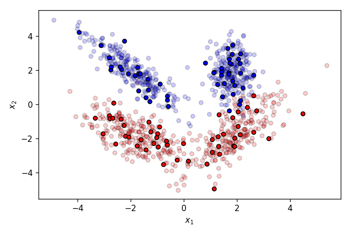
Let's create a dataset slightly more complicated than the one above.
X,y = make_classification(n_samples=1000, n_features=2, n_informative=2,
                    n_redundant=0, n_repeated=0, n_classes=2, n_clusters_per_class=2,
                          class_sep=1.8,
                   flip_y=0,weights=[0.5,0.5], random_state=580)

fig = plt.figure(dpi=120)
plot_points(X,y,alpha=.8)
plt.savefig('1.png')
plt.show()

This time, the features of the pets have a much more complicated relationship with the output classes cat and dog. As it's clearly obvious from the graph above, this dataset cannot be properly segmented by a linear decision boundary. This is where a Multilayer Perceptron (MLP) comes into picture.
Multilayer Perceptron
A multilayer perceptron (MLP) is a class of feedforward artificial neural networks. As the name suggests, it's comprised of multiple neurons stacked together. The following is one of the simplest MLPs possible.
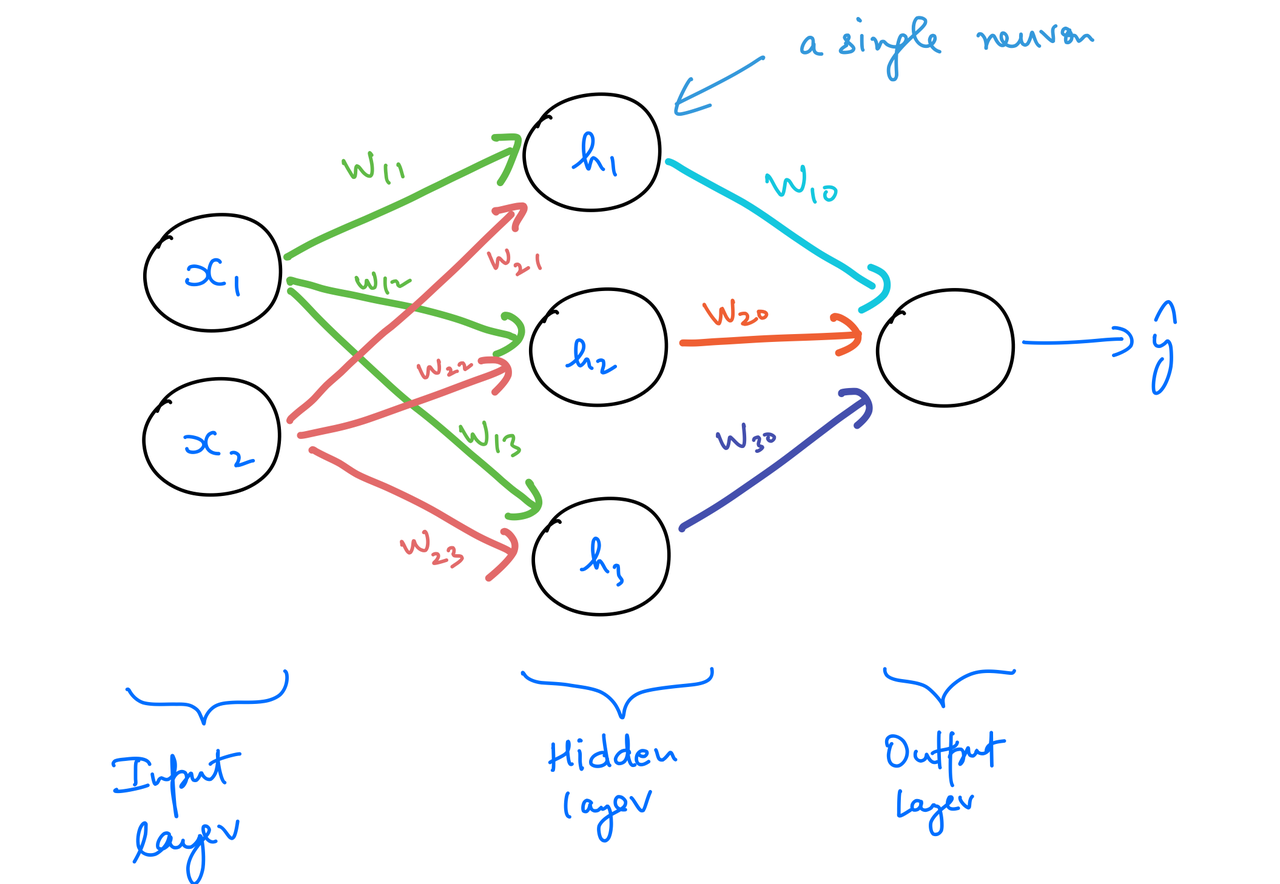
The MLP above has 4 neurons in it, with 3 being in the hidden layer, and one in the output layer. The input layer is a simple one-to-one mapping with the input features. Let's try to understand the reasoning behind stacking them up like this.
Instead of having one neuron perform a weighted sum of the inputs, we'll make the 3 neurons in the hidden layer perform the same task. Each neuron has its own sets of weights and biases associated with it. The weighted sum is then passed on to a non-linear activation function (sigmoid in this case).
Till now in the process, it's like having 3 different neurons do the same task independently. The gamechanger is to then have the outputs of these 3 neurons be input to the neurons of the next layer (a single neuron in this case). This output neuron performs a weighted sum of the activations input to it, and passes them through a non-linear function. Since, we want the output of the model to be probabilities, we'll use sigmoid as the activation function. The whole process is termed as feedforward operation.
Feedforward
Let's see how the feedforward operation is performed in an MLP.
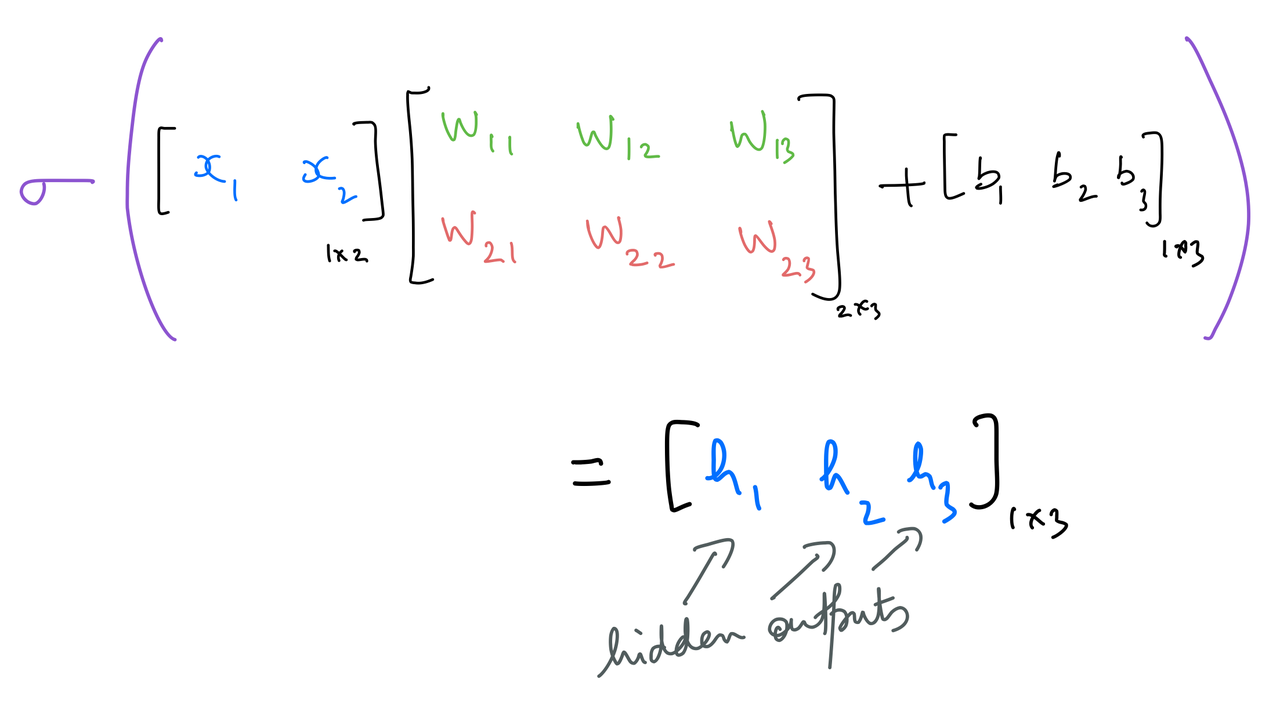
The neurons of the hidden layer have their weights and biases. The weights can be represented as the following matrix:
$$ \large \text{weightsInputToHidden} = \begin{bmatrix} w_{11} & w_{12} & w_{13} \\ w_{21} & w_{22} & w_{23} \end{bmatrix} $$N_input = 2
N_hidden = 3
N_output = 1
weights_input_to_hidden = np.random.normal(0, scale=0.1, size=(N_input, N_hidden))
weights_input_to_hidden
bias_input_to_hidden = np.zeros(N_hidden)
bias_input_to_hidden
Hidden outputs
The hidden outputs are calculated as follows:
def sigmoid(x):
    return 1/(1+np.exp(-x))
input_x = X[0,:].reshape(1,-1)
input_x.shape
output_y = y[0].reshape(1,-1)
output_y.shape
hidden_layer_in = np.dot(input_x,weights_input_to_hidden) + bias_input_to_hidden
hidden_layer_out = sigmoid(hidden_layer_in)
hidden_layer_out
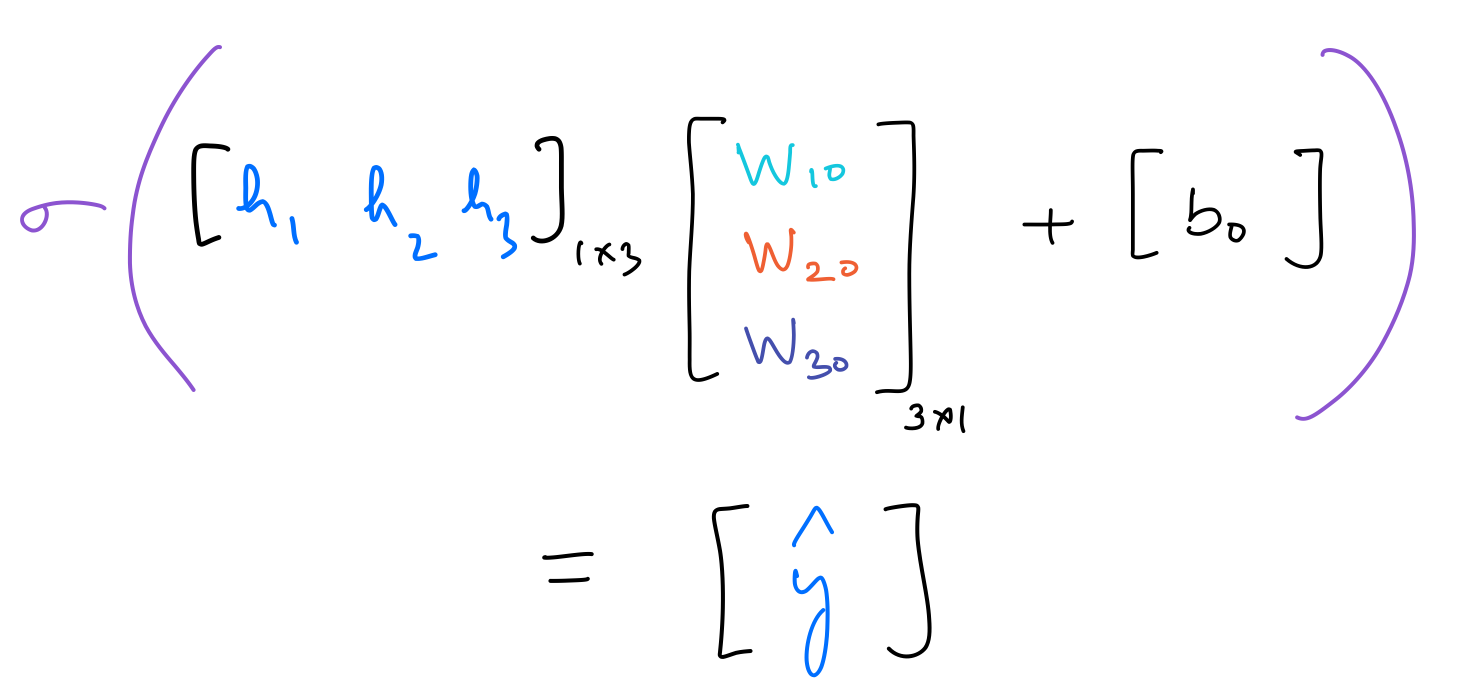
Next, the output neuron has its set of weights and bias. This can be represented as:
$$ \large \text{weightsHiddenToOutput} =\begin{bmatrix} w_{1o}\\w_{2o}\\w_{3o} \end{bmatrix} $$weights_hidden_to_output = np.random.normal(0, scale=0.1, size=(N_hidden, N_output))
weights_hidden_to_output
bias_hidden_to_output = np.zeros(N_output)
bias_hidden_to_output
Output
The operation performed by the output neuron is as follows:
output_layer_in = np.dot(hidden_layer_out,weights_hidden_to_output) + bias_hidden_to_output
output_layer_out = sigmoid(output_layer_in)
output_layer_out
Error Function
As we know from the last post, binary cross-entropy is used to calculate error for binary classification problems. Binary cross-entropy for a single data point is as follows: $$ \large E = -y\log(\hat{y}) - (1-y)\log(1-\hat{y}) $$
error = (-1)*output_y*np.log(output_layer_out) - (1-output_y)*np.log(1-output_layer_out)
error
In order to have the MLP properly model the dataset, this error needs to be minimised. As we'll see below, this can be done through gradient descent.
Backpropagation
Since the prediction of the MLP is a function of all the parameters of the MLP — weights_input_to_hidden, bias_input_to_hidden, weights_hidden_to_output, and bias_hidden_to_output — the error is a function of these parameters too.
Thus, it can be minimised by performing gradient descent as follows: $$ \large parameter \leftarrow parameter - \alpha\frac{\partial E}{\partial parameter} $$
Partial derivative wrt prediction
Let's start by calculating the partial derivative of the error wrt. the output prediction $\hat{y}$.
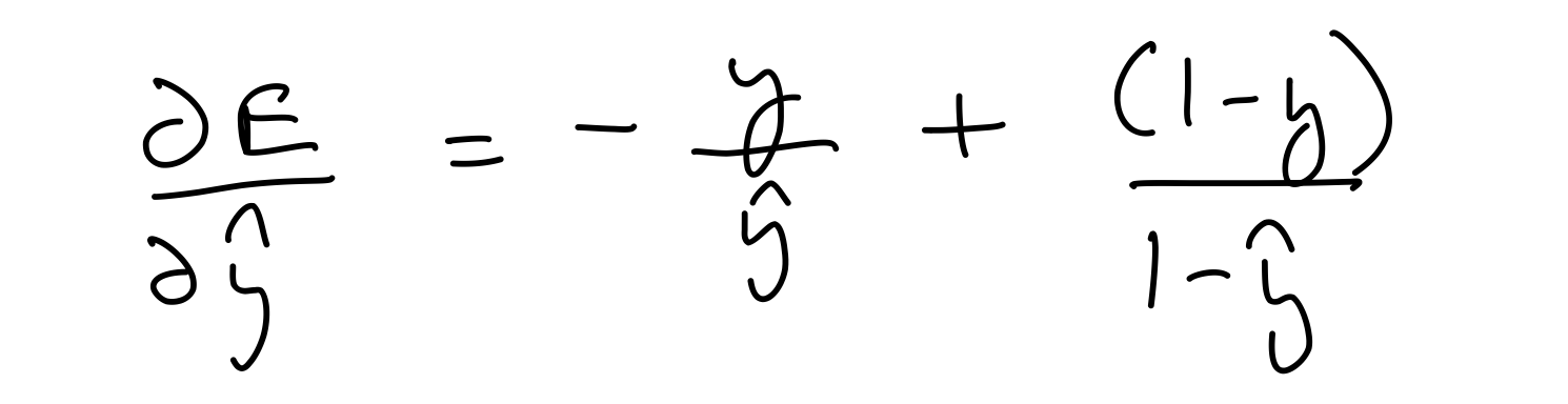
del_y_out = (-1)*output_y/output_layer_out + (1-output_y)/(1-output_layer_out)
del_y_out
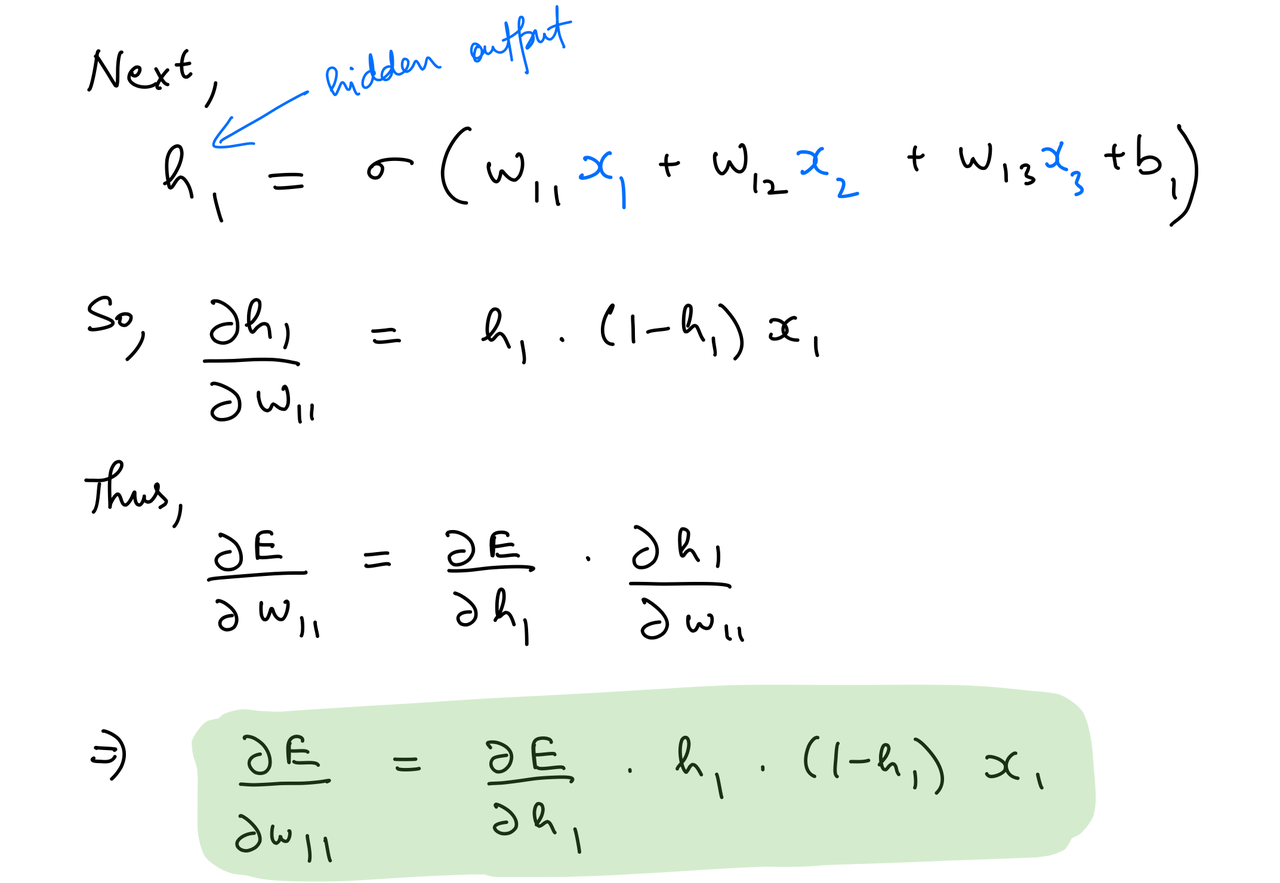
Partial derivate wrt hidden output
We can then calculate the partial derivative of the error wrt to the other parameters by using the chain rule.
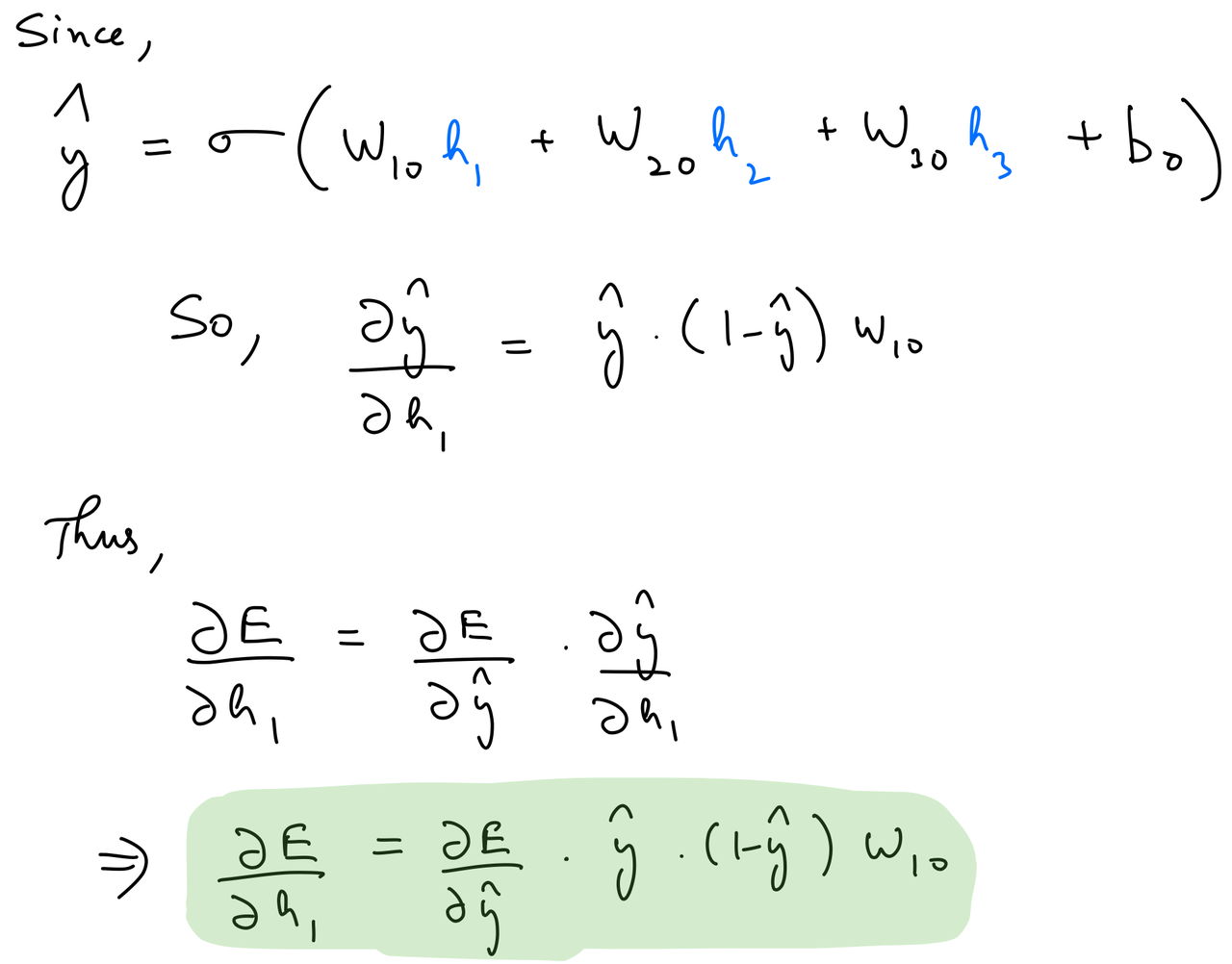
del_h = del_y_out*output_layer_out*(1-output_layer_out)*weights_hidden_to_output.T
del_h
Partial derivative wrt output layer weights
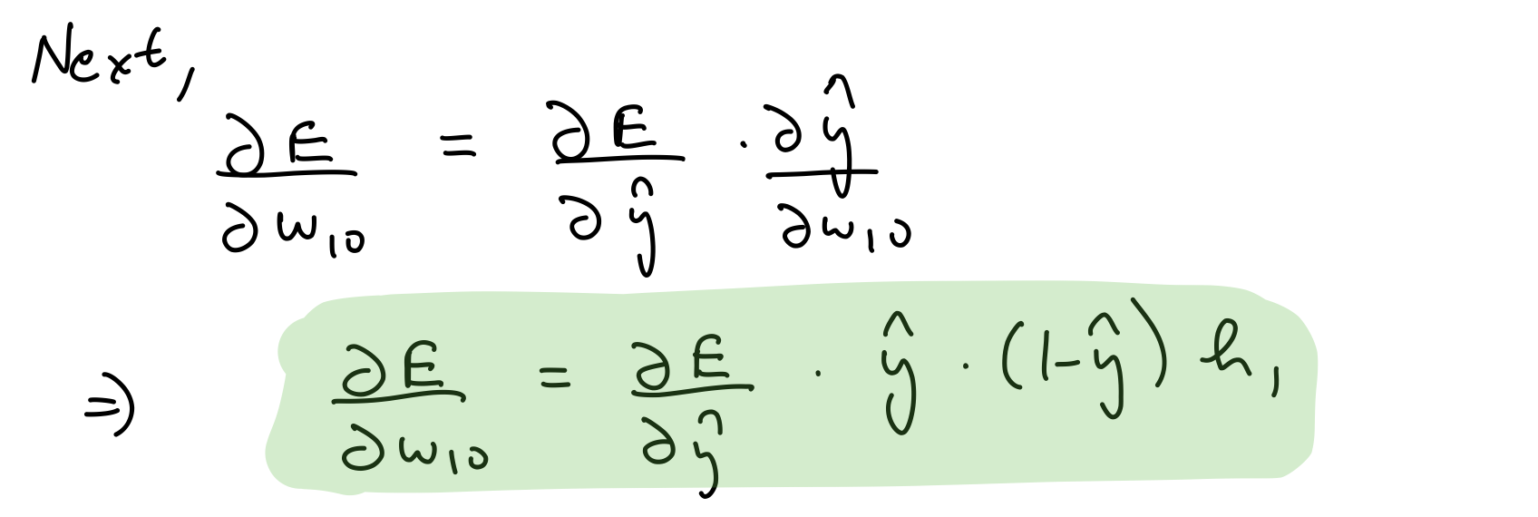
del_w_h_o = del_y_out*output_layer_out*(1-output_layer_out)*hidden_layer_out.T
del_w_h_o
Partial derivative wrt output layer biases
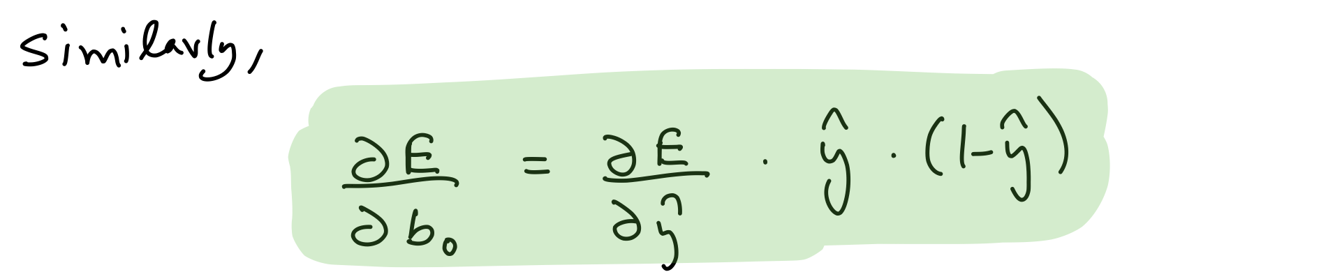
del_b_o = del_y_out*output_layer_out*(1-output_layer_out)
del_b_o
Partial derivative wrt hidden layer weights
del_w_i_h = del_h*hidden_layer_out*(1-hidden_layer_out)*input_x.T
del_w_i_h
Partial derivative wrt hidden layer biases
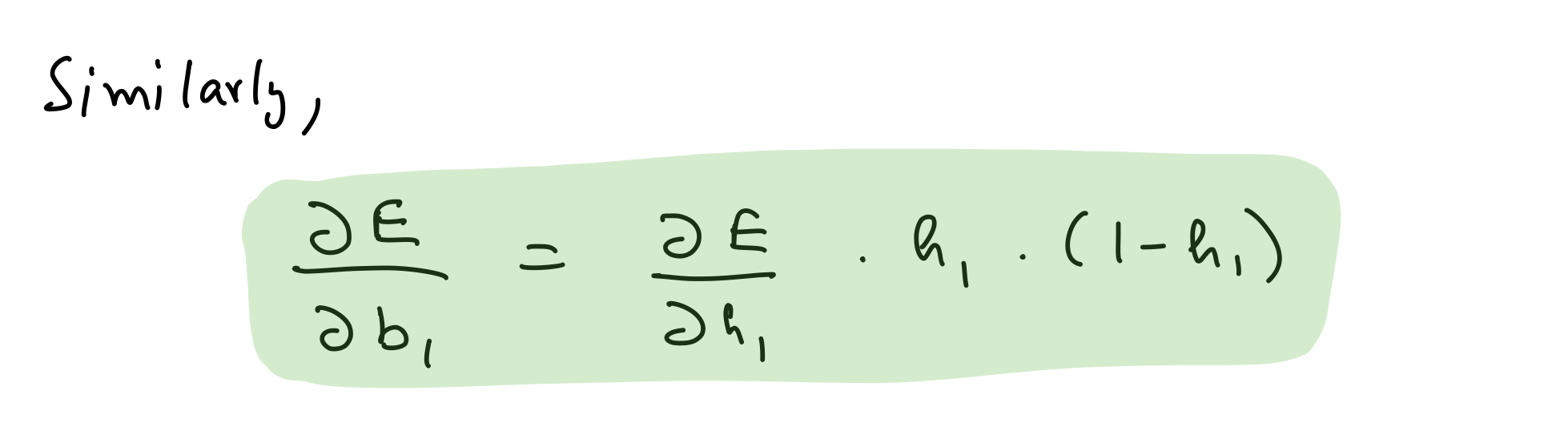
del_b_h = del_h*hidden_layer_out*(1-hidden_layer_out)
del_b_h
Let's perform the gradient descent step, with an appropriate learning rate.
learn_rate = 1e-3
# update
weights_hidden_to_output -= learn_rate*del_w_h_o
bias_hidden_to_output -= learn_rate*del_b_o[0,:]

weights_input_to_hidden -= learn_rate*del_w_i_h
bias_input_to_hidden -= learn_rate*del_b_h[0,:]
This is how backpropagation works in an MLP, and neural networks in general.
Let's put all of this in a single class titled MLPNeuralNet, with it's own implementaions of forward propagation (feed_forward), and backpropagation (back_propagate).
class MLPNeuralNet(object):
    def __init__(self,N_input, N_hidden,N_output):
        self.weights_input_to_hidden = np.random.normal(0, scale=0.1, size=(N_input, N_hidden))
        self.weights_hidden_to_output = np.random.normal(0, scale=0.1, size=(N_hidden, N_output))

        self.bias_input_to_hidden = np.zeros(N_hidden)
        self.bias_hidden_to_output = np.zeros(N_output)


    def feed_forward(self,input_x):
        self.hidden_layer_in = np.dot(input_x,self.weights_input_to_hidden) + self.bias_input_to_hidden
        self.hidden_layer_out = sigmoid(self.hidden_layer_in)
        self.output_layer_in = np.dot(self.hidden_layer_out,self.weights_hidden_to_output) + self.bias_hidden_to_output
        self.output_layer_out = sigmoid(self.output_layer_in)
        return self.output_layer_out

    def back_propagate(self,input_x,output_y, learn_rate):
        error = (-1)*(output_y*np.log(self.output_layer_out) + (1-output_y)*np.log(1-self.output_layer_out))
        del_y_out = (-1)*output_y/self.output_layer_out + (1-output_y)/(1-self.output_layer_out)
        del_h = del_y_out*self.output_layer_out*(1-self.output_layer_out)*self.weights_hidden_to_output.T
        del_w_h_o = del_y_out*self.output_layer_out*(1-self.output_layer_out)*self.hidden_layer_out.T
        del_b_o = del_y_out*self.output_layer_out*(1-self.output_layer_out)
        del_w_i_h = del_h*self.hidden_layer_out*(1-self.hidden_layer_out)*input_x.T
        del_b_h = del_h*self.hidden_layer_out*(1-self.hidden_layer_out)

        self.weights_hidden_to_output -= learn_rate*del_w_h_o
        self.bias_hidden_to_output -= learn_rate*del_b_o[0,:]

        self.weights_input_to_hidden -= learn_rate*del_w_i_h
        self.bias_input_to_hidden -= learn_rate*del_b_h[0,:]
        return error
Training
Let's write a training function that will run gradient descent on a MLPNeuralNet object.
def train(nn, features, outputs, num_epochs, learn_rate, print_error=False):

    for e in range(num_epochs):
        for input_x, output_y in zip(features, outputs):
            input_x = input_x.reshape(1,-1)
            output_y = output_y.reshape(1,-1)

            output_layer_out = nn.feed_forward(input_x)

            error = nn.back_propagate(input_x,output_y,learn_rate)

        if print_error:
            if e%200==0:
                print(error[0][0])
Let's divide up the datasets into training and validation sets.
np.random.seed(10)
indices = np.random.permutation(X.shape[0])
training_idx, validation_idx = indices[:900], indices[900:]
training_set_features, validation_set_features = X[training_idx,:], X[validation_idx,:]
training_set_labels, validation_set_labels = y[training_idx], y[validation_idx]
training_set_features.shape,training_set_labels.shape
validation_set_features.shape,validation_set_labels.shape
Let's plot the two sets. The transparent data points belong to the training set, while the others belong to the validation set.
fig=plt.figure(dpi=120)
plot_points(training_set_features,training_set_labels,alpha=.2)
plot_points(validation_set_features,validation_set_labels,alpha=1.)
plt.legend().set_visible(False)
plt.savefig('2.png')
plt.show()
Training the MLP on the training set.
np.random.seed(10)
nn = MLPNeuralNet(N_input, N_hidden, N_output)
train(nn,training_set_features,training_set_labels,2000,1e-3,print_error=True)
Let's see how well the model performs on the validation set.
((nn.feed_forward(validation_set_features)>=0.5).astype(int)==validation_set_labels.reshape(-1,1)).mean()*100
It's correctly classifying points in the validation set with a 97% accuracy. That's pretty good. Let's see the decision boundary for the MLP after training.
Decision Boundary
Let's see how well the MLP models the dataset.
h = .02
x_min, x_max = X[:, 0].min() - 1, X[:, 0].max() + 1
y_min, y_max = X[:, 1].min() - 1, X[:, 1].max() + 1
xx, yy = np.meshgrid(np.arange(x_min, x_max, h),
                     np.arange(y_min, y_max, h))

Z = (nn.feed_forward(np.c_[xx.ravel(), yy.ravel()]) >0.5).astype(int)

Z = Z.reshape(xx.shape)
fig = plt.figure(dpi=150)
plt.contourf(xx, yy, Z, cmap=plt.cm.RdBu)
plot_points(X,y,alpha=.8)
plt.title('Solution Boundary');
plt.savefig('3.png')
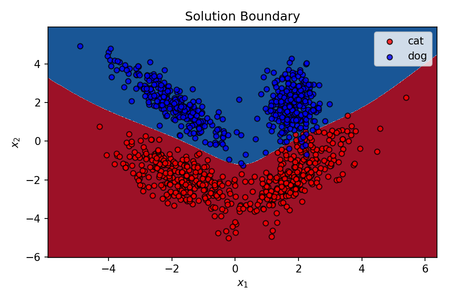
That's pretty good for this super simple MLP with only 4 neurons. As I mentioned before, the capability of a MLP of creating non-linear decision boundary comes from it's constituent neurons learning different decision boundaries of their own, and the output prediction being influenced by each of these individual decision boundaries by different weightages. These weights connecting different neurons are optimised by backpropagation during gradient descent.
Let's take a look at how the decision boundary of the MLP, as well as the decision boundaries of the neurons in the hidden layer shape up during the training process.
def display_linear_boundary(ax, m, b, x_1_lims,x_2_lims,color='g--',label=None,linewidth=3.):
    ax.set_xlim(x_1_lims)
    ax.set_ylim(x_2_lims)
    x = np.arange(-10, 10, 0.1)
    ax.plot(x, m*x+b, color, label=label,linewidth=linewidth)
    ax.set_yticklabels([])
    ax.set_xticklabels([])
    return ax
def plot_points_on_ax(ax,X, y,alpha):
    dogs = X[np.argwhere(y==1)]
    cats = X[np.argwhere(y==0)]
    ax.scatter([s[0][0] for s in cats], [s[0][1] for s in cats], s = 25, \
               color = 'red', edgecolor = 'k', label='cats',alpha=alpha)
    ax.scatter([s[0][0] for s in dogs], [s[0][1] for s in dogs], s = 25, \
               color = 'blue', edgecolor = 'k', label='dogs',alpha=alpha)
    return ax
def create_decision_boundary_anim(nn,X,y,epochs=300,learn_rate=1e-3,snap_every=100,dpi=100,print_error=False):

    fig = plt.figure(figsize=(9,9),dpi=dpi)

    gs = fig.add_gridspec(3, 3)

    sol_bound = fig.add_subplot(gs[:2, :])
    sol_bound.set_yticklabels([])
    sol_bound.set_xticklabels([])

    h_1 = fig.add_subplot(gs[2, 0])

    h_2 = fig.add_subplot(gs[2, 1])

    h_3 = fig.add_subplot(gs[2,2])

    hidden_layer_axes = [h_1, h_2, h_3]


    camera = Camera(fig)

    h = .02

    x_min, x_max = X[:, 0].min() - 1, X[:, 0].max() + 1
    y_min, y_max = X[:, 1].min() - 1, X[:, 1].max() + 1
    xx, yy = np.meshgrid(np.arange(x_min, x_max, h),
                     np.arange(y_min, y_max, h))


    for e in range(ceil(epochs/snap_every)):
        train(nn,X,y,snap_every,learn_rate,print_error=print_error)
        Z = (nn.feed_forward(np.c_[xx.ravel(), yy.ravel()]) >0.5).astype(int)
        Z = Z.reshape(xx.shape)
        sol_bound.contourf(xx, yy, Z, cmap=plt.cm.RdBu)

        for i,ax in enumerate(hidden_layer_axes):

            w1,w2 = nn.weights_input_to_hidden[:,i][0],nn.weights_input_to_hidden[:,i][1]
            b = nn.bias_input_to_hidden[i]

            ax = display_linear_boundary(ax, -w1/w2, -b/w2, [x_min, x_max], [y_min, y_max])

        text_box = AnchoredText(f'Epoch: {snap_every*(e+1)}', frameon=True, loc=4, pad=0.5)
        plt.setp(text_box.patch, facecolor='white', alpha=0.5)
        sol_bound.add_artist(text_box)

        camera.snap()


    sol_bound = plot_points_on_ax(sol_bound,X, y,alpha=.6)
    sol_bound.set_title(f'Decision boundary of MLP')

    for i,ax in enumerate(hidden_layer_axes):
        ax = plot_points_on_ax(ax,X, y,alpha=.6)
        ax.set_title(f'Hidden neuron {i+1}')

    plt.tight_layout()
    animation = camera.animate()

    return animation
np.random.seed(10)
nn = MLPNeuralNet(N_input, N_hidden, N_output)
anim = create_decision_boundary_anim(nn,training_set_features,training_set_labels,\
                                     epochs=2000,dpi=120,\
                                     learn_rate=1e-3,snap_every=50,\
                                     print_error=False)
plt.close()
HTML(anim.to_html5_video())
Let's increase the learning rate to 5e-5. This will speed up the training process as evident below.
np.random.seed(10)
nn = MLPNeuralNet(N_input, N_hidden, N_output)
anim = create_decision_boundary_anim(nn,training_set_features,training_set_labels,\
                                     epochs=500,dpi=120,\
                                     learn_rate=5e-3,snap_every=50,\
                                     print_error=False)
plt.close()
HTML(anim.to_html5_video())
The larger cell shows the evolution of the MLP's decision boundary during the training process. The bottom 3 cells show the decision boundaries of the 3 neurons in the hidden layer.
It can be seen in the animation above that the decision boundaries of the 3 neurons come together to create the non-linear decision boundary of the MLP. The curviness of the decision boundary increases as those of neurons 1 and 3 become steeper.
This is how neurons — when properly stacked together — can create neural networks that can learn to segment datasets that are not linearly separable.